


















Lesson 35 of 49 · Panel Data and Time Series
Fixed and random effects
Understand pooled OLS, the within (fixed effects) estimator, first differences and random effects, and choose between them with the Hausman test.
Return to the firms and their advertising. You observe 200 firms for six years. What causes the differences in profit that are not explained by advertising? Some of it is year-to-year luck, which changes constantly. But a big part is a firm's lasting quality: the strength of its brand, the skill of its managers, the neighbourhood it operates in. These traits are real, they affect profit, and they are probably correlated with how much the firm advertises. They are also (mostly) constant over the six years.
Panel methods exploit exactly this combination. In this lesson you will write down the error-components model, see why pooled OLS can fail, learn the fixed-effects and random-effects estimators, and compare them with the Hausman test.
What you will learn
- The error-components model
yit = xit'β + αi + uit. - Why pooled OLS is inconsistent when the unit effect is correlated with the regressors.
- How the within (fixed effects) transformation and first differencing remove
αi. - How random effects works, when it is more efficient, and how the Hausman test chooses.
Key terms
Unit effect αi: all time-invariant influences on the unit's outcome, observed or not. Idiosyncratic error uit: the part that varies over time. Within transformation: subtracting each unit's time average from every variable. Random effects: the assumption that αi is uncorrelated with all regressors. Cluster-robust standard errors: standard errors that allow arbitrary correlation of errors within a unit.
The model
The workhorse specification is
yit = β0 + β1 xit + αi + uit, i = 1, ..., N, t = 1, ..., T
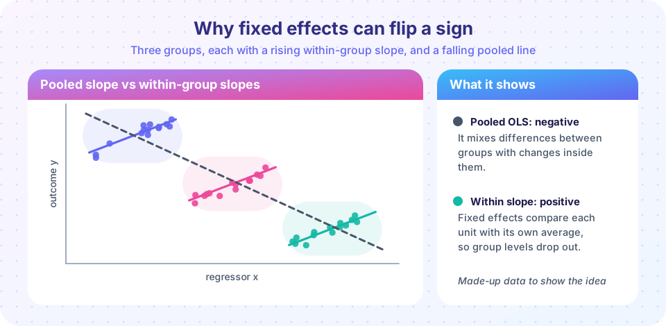
Here αi is the unit effect and uit the idiosyncratic error. The composite error is vit = αi + uit. Two consequences follow immediately. First, the composite error is correlated within a unit, because every period shares the same αi; the correlation between two errors of the same unit is σα² / (σα² + σu²). This means the usual standard errors are wrong, a problem reminiscent of chapter 5. Second, if αi is correlated with xit, then Cov(xit, vit) ≠ 0: the regressor is endogenous, and pooled OLS (stacking all observations and running OLS) is inconsistent.
Fixed effects: the within estimator
Average the model over time for unit i:
ȳi = β0 + β1 x̄i + αi + ūi
and subtract it from the original equation. The unit effect cancels:
(yit − ȳi) = β1 (xit − x̄i) + (uit − ūi)
Estimate β1 by OLS on these demeaned variables. That is the fixed-effects (within) estimator. It needs only that uit is uncorrelated with xis for all periods (strict exogeneity). It does not matter how αi relates to xit.
An equivalent route is the least-squares dummy variable (LSDV) estimator: include a dummy for every unit. By the Frisch-Waugh-Lovell theorem the slope is identical. The dummy approach makes the cost visible: you estimate N extra parameters. The within version computes them away, but you must remember to correct the degrees of freedom: NT − N − k, not NT − k. Good software does this for you.
Two important side effects:
- Time-invariant regressors drop out. Gender, a country's geography or a firm's founding year are constant within a unit, so after demeaning they are zero. Fixed effects cannot estimate their coefficients; it can only control for them.
- Only within variation matters. If a variable barely changes within units, its coefficient is imprecise.
A related estimator is first differencing: subtract the previous period, Δyit = β1 Δxit + Δuit. With T = 2 it is identical to fixed effects. For T > 2 the two differ; first differences are preferable when uit is close to a random walk, while fixed effects are more efficient when uit is serially uncorrelated.
You can also add time effects (year dummies) to control for shocks common to all units, such as a recession, giving the two-way fixed effects model.
Random effects
If you believe αi is uncorrelated with every regressor, fixed effects is unnecessarily costly: it throws away the between variation. The random-effects estimator uses both. It is a generalized least squares (GLS) estimator that exploits the known error structure by quasi-demeaning:
(yit − θ ȳi) = β0 (1 − θ) + β1 (xit − θ x̄i) + (error), with θ = 1 − √( σu² / (σu² + T σα²) )
When θ = 0 you get pooled OLS; when θ = 1 you get the within estimator. In practice θ lies in between and approaches 1 as T grows or as unit heterogeneity σα² grows. Random effects is more efficient than fixed effects when its assumption holds, and it can estimate coefficients of time-invariant regressors. If the assumption fails, it is inconsistent.
Choosing: the Hausman test
If αi is uncorrelated with x, both FE and RE are consistent, and RE is efficient. If not, only FE is consistent. The Hausman test exploits this: under the null, the two estimates should be close. The statistic for a single coefficient is
H = (b_FE − b_RE)² / (Var(b_FE) − Var(b_RE)), distributed chi-square with 1 degree of freedom under the null
(with several regressors, a quadratic form in the coefficient differences). Rejection says: the random-effects assumption is violated, use fixed effects. Failure to reject says there is no strong evidence against RE. A robust alternative is the Mundlak (or correlated random effects) approach: add the unit averages x̄i to the RE regression; if their coefficients are zero, RE is fine. Because the classical Hausman test needs homoskedastic errors and an efficient RE, applied researchers often use this regression-based version with cluster-robust standard errors.
Practical rule: in observational economic data, αi is usually correlated with the regressors, so fixed effects is the default. Random effects makes most sense when units are randomly sampled from a large population and you care about time-invariant variables, or in designs where assignment is random.
Standard errors: cluster by unit
With panel data, errors within a unit are correlated over time (through αi and often serial correlation in uit). The remedy is cluster-robust standard errors, clustered at the unit level, which allow arbitrary correlation within each unit and arbitrary heteroskedasticity. They are the default for panel regressions and are valid when the number of clusters is reasonably large (a few dozen or more).
Seeing the estimators disagree
We simulate a panel in which the unit effect is correlated with x, so the truth is 0.5: pooled OLS and random effects are biased, fixed effects is right. In the second scenario, the unit effect is unrelated to x, and RE and FE agree.
Press Run (or Ctrl + Enter) to see the result here.
Program input · what you'd type while the program runs
Type the answers before you press Run, one per line. Each time the program reads a line (with input()), it gets the next line from this box.
In the first scenario pooled and RE sit above 0.5 while FE and FD are near it, and the Hausman statistic is large. In the second, all four estimators are close and H is small.
Visualizing the within transformation
Press Run (or Ctrl + Enter) to see the result here.
Program input · what you'd type while the program runs
Type the answers before you press Run, one per line. Each time the program reads a line (with input()), it gets the next line from this box.
Left: the pooled line slopes downward because high-α units have low x. Right: after demeaning, the three clouds are stacked on top of each other, and the within slope recovers the truth.
Common misconceptions
"Fixed effects estimates the effect of time-invariant variables." It cannot: those variables are wiped out by demeaning.
"Random effects is always better because it is more efficient." Efficiency means nothing if the estimator is inconsistent. If αi is correlated with the regressors, RE is biased.
"A significant Hausman test means fixed effects is correct." It means RE's assumption is rejected; FE still needs strict exogeneity of uit.
"Clustering fixes everything." It repairs standard errors, not endogeneity from time-varying confounders.
Check your understanding
Quick check · 5 questions
of 5 answered You scored / 5 · perfect!
-
1. What does the within transformation subtract from each variable?
Subtracting each unit's own mean removes anything constant over time, including the unit effect. -
2. Which regressor CANNOT be estimated by a fixed-effects model?
A time-invariant variable is constant within a unit and disappears after demeaning. -
3. When theta = 1 in the random-effects transformation, RE equals...
Quasi-demeaning with theta = 1 subtracts the full unit mean, which is the within transformation. -
4. A significant Hausman test indicates that...
The test compares FE and RE; a large difference means alpha is correlated with the regressors. -
5. Why should panel standard errors usually be clustered by unit?
The unit effect and serial correlation make errors within a unit dependent.
Summary
- The model
yit = xit'β + αi + uitexplains why pooled OLS fails whenαiis correlated withx. - Fixed effects demeans by unit (or adds unit dummies); it removes unobserved time-invariant traits but cannot estimate time-invariant regressors.
- Random effects quasi-demeans and is efficient only if
αiis uncorrelated with the regressors; the Hausman or Mundlak test checks this. - Cluster standard errors by unit.
Track your progress
Create a free account to tick off lessons and pick up where you left off on any device.
of Econometrics lessons completed