


















Lesson 44 of 49 · Projects and Practice
Project: diagnosing a wage regression
A hands-on project: fit a wage equation, plot residuals, run Breusch-Pagan and White tests, compare standard errors and write a short, honest results table.
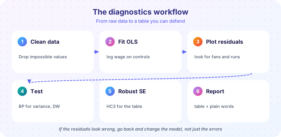
This project puts chapters 2 to 5 to work on the most traditional regression in applied economics: a wage equation relating pay to schooling, experience and gender. You will not only estimate it. You will interrogate it, step by step, the way a referee would, and end with a short results table and a paragraph of plain-language interpretation.
The data are invented and simulated inside the code, so that you know the truth and can check whether each diagnostic finds what we planted. That is a useful habit in its own right: simulate first, then trust the tool on real data.
What you will learn
- How to run an end-to-end diagnostic workflow on a regression.
- How to read residual plots and tests together, and decide what to do.
- How to compare usual, robust and weighted estimates in one table.
- How to write the result so that a reader can audit it.
Key terms
Mincer equation: a log wage regression on schooling and a quadratic in experience, named after Jacob Mincer. Return to schooling: the percentage change in wages for one more year of education, 100 × β for small β. Diagnostics: checks that residuals behave as the assumptions require. Robust standard errors: valid under uneven error variance. Results table: coefficients with standard errors, the sample size and the method.
The model
Following Mincer (1974), the benchmark specification is
log(wage) = β0 + β1 educ + β2 exper + β3 exper² + β4 female + u
Taking logs has three attractions: the coefficient on educ reads as an approximate percentage return, wages are right-skewed and logs make them closer to symmetric, and the error variance in a log equation is usually more stable than in a level equation. The squared experience term allows wages to rise with experience at a decreasing rate: the effect of one more year is β2 + 2 β3 exper.
Remember what this regression does not identify. Schooling is probably correlated with unobserved ability, so β1 may overstate the causal return (chapter 6). The project is about diagnostics of the regression you did run, not a claim that it is causal.
Step 1: build the data and fit OLS
In the simulated data, the true return to schooling is 0.08, the true female gap is −0.12 log points, and the error variance grows with years of schooling (more educated workers have more variable wages). That planted pattern is the heteroskedasticity your diagnostics should find.
Press Run (or Ctrl + Enter) to see the result here.
Program input · what you'd type while the program runs
Type the answers before you press Run, one per line. Each time the program reads a line (with input()), it gets the next line from this box.
Read the output in order. The tests should reject constant variance decisively. The OLS and WLS coefficients should both be close to the truth (0.08 for educ), the usual and robust standard errors for educ should differ noticeably, and the female gap should be near −0.12.
Step 2: look at the residuals
Tests answer "is there a pattern?" but only a picture tells you what the pattern is. Plot the residuals against the fitted values and, more informatively, the average absolute residual by years of schooling. Then repeat the exercise for a regression on the level of the wage, to see why the log specification is preferred.
Press Run (or Ctrl + Enter) to see the result here.
Program input · what you'd type while the program runs
Type the answers before you press Run, one per line. Each time the program reads a line (with input()), it gets the next line from this box.
In the left panel the log-wage residuals show a mild widening to the right; the middle panel reveals the planted pattern directly: the typical error grows steadily with schooling. The right panel shows what happens in levels: a much stronger funnel, because a percentage shock is a bigger dollar amount for a higher wage. This is a typical reason to prefer the log form.
Step 3: read the tests and decide
Put the evidence together before you choose a repair.
| Evidence | What it says |
|---|---|
| Residual plot, mean absolute residual by schooling | Spread rises with schooling |
| Breusch-Pagan and White (special case) | Reject constant variance |
Usual versus HC3 standard error on educ |
They differ, so inference is affected |
| OLS versus WLS coefficients | Similar, as expected when the mean equation is right |
Decision: keep the log specification, report OLS coefficients with HC3 standard errors as the headline, and show WLS as a robustness check. Report the usual standard errors in a note or an appendix so the reader can see the size of the difference.
What would you do differently if the OLS and WLS coefficients differed a lot? That is a warning that the mean equation may be misspecified (a missing interaction, say between education and experience): WLS and OLS estimate the same thing only if the model is correct. Investigate the functional form before choosing between them.
Step 4: write the results table
A clear table has coefficients, standard errors in parentheses, the type of standard error, the sample size and a note on what is being estimated. For example:
| (1) OLS, usual SE | (2) OLS, HC3 SE | (3) WLS | |
|---|---|---|---|
| Years of education | β̂ (se) | β̂ (se) | β̂ (se) |
| Experience | … | … | … |
| Experience squared | … | … | … |
| Female | … | … | … |
| Observations | 1,500 | 1,500 | 1,500 |
Notes: dependent variable is the log hourly wage; HC3 standard errors in column 2; WLS weights come from a regression of the log squared residual on education. Fill in the numbers from your own run.
The paragraph beneath the table should answer four questions in plain words: what is the estimated return to schooling and how precise is it; how large is the female gap; what did the diagnostics find; and what is not shown (for example, that the schooling return is not necessarily causal).
Your turn
Extend the project in at least two of these directions, running each in the editor above.
- Interaction. Add
educ × femaleand test whether the return to schooling differs by gender. - Functional form. Replace
exper + exper²with a cubic and use an F test (chapter 4) to see if it improves the fit. - Different weights. Assume the variance depends on both schooling and experience; build the FGLS weights from a regression of
log(e²)on both. - Clustering. Suppose workers are grouped into 50 firms and errors within a firm share a common component. Add a firm effect to the simulation and compare the usual, HC3 and cluster-robust standard errors.
- Stress test. Change the planted standard deviation to a constant and confirm that the tests no longer reject (about 5% of the time they will, by chance).
Common misconceptions
"A significant Breusch-Pagan test means my coefficients are wrong." It means the usual standard errors are unreliable. The coefficients are still unbiased under the exogeneity assumption.
"Robust standard errors always give a smaller p-value." They can go either way; the aim is validity.
"If the residual plot looks fine, I do not need to report robust errors." Reporting robust errors by default costs little and protects you from patterns that plots hide in large samples.
Check your understanding
Quick check · 5 questions
of 5 answered You scored / 5 · perfect!
-
1. Why is a log wage equation usually preferred to a level wage equation?
Logs give a percentage interpretation, reduce skewness and often tame heteroskedasticity. -
2. The experience effect in the Mincer equation is beta2 + 2 beta3 exper. If beta3 is negative, the effect of an extra year of experience...
A negative quadratic term makes returns to experience diminishing. -
3. The Breusch-Pagan test rejects. The best next step is...
Rejection concerns the variance; robust errors repair inference and the plot shows the form. -
4. OLS and WLS coefficients differ hugely. This suggests...
If the model is right, both are consistent for the same parameters; a big gap signals misspecification. -
5. Why should the usual standard errors also be shown, perhaps in a note?
Showing both makes the correction transparent and checkable.
Summary
- A diagnostic workflow runs from a clean fit to residual plots, formal tests, robust or modelled errors and an honest write-up.
- Plots show the form of a problem; tests quantify it; robust standard errors are the safe default for cross-sections.
- Compare usual, robust and weighted results, and treat big discrepancies as a sign to revisit the model.
- State what the regression does not identify (here, causality of schooling).
Track your progress
Create a free account to tick off lessons and pick up where you left off on any device.
of Econometrics lessons completed