


















Lesson 37 of 49 · Panel Data and Time Series
Cointegration, error correction and forecasting
Avoid spurious regression with cointegration: the Engle-Granger two-step test, the error correction model, and a first look at forecasting with AR models.
The last lesson ended with an uncomfortable message: regressing one unit-root series on another can produce nonsense. Yet economic theory is full of long-run relationships among trending variables. Consumption and income track each other. Prices of the same good in two cities do not drift apart forever. Short-term and long-term interest rates move together. If these links are real, a regression in levels is not nonsense; it is the best way to estimate them.
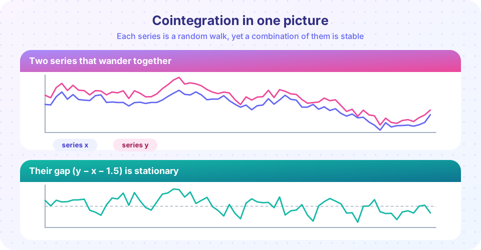
Cointegration (Granger, 1981; Engle and Granger, 1987) resolves the apparent paradox. Two series can each wander without direction, yet a specific combination of them can be stable. This lesson explains how to detect it with the Engle-Granger test, how to model both long-run and short-run behaviour with an error correction model, and how to use stationary models for forecasting.
What you will learn
- Why regressing unit-root series on each other is dangerous, and a quick warning sign.
- The definition of cointegration and the Engle-Granger two-step procedure.
- How an error correction model links short-run changes to the long-run gap.
- How AR forecasts behave over time, and how to compare forecast accuracy.
Key terms
Spurious regression: a regression of independent I(1) series that nonetheless gives a "significant" slope and a high R². Cointegration: I(1) series for which some linear combination is I(0). Cointegrating vector: the coefficients of that combination. Error correction: short-run adjustment toward the long-run relationship. Forecast horizon h: the number of periods ahead being predicted.
Spurious regression and a rule of thumb
Granger and Newbold (1974) generated independent random walks and regressed one on the other, finding "significant" t statistics in most trials. The residuals of such a regression are themselves nonstationary: highly persistent, with a very low Durbin-Watson statistic. Their rule of thumb: if R² is larger than the Durbin-Watson statistic, suspect a spurious regression. The modern advice is simply: never interpret levels regressions of unit-root series without testing for cointegration.
Cointegration
Suppose xt and yt are both I(1). Generally any combination yt − β xt is also I(1). If for some special β the combination
zt = yt − β xt
is I(0), then x and y are cointegrated with cointegrating vector (1, −β). Interpretation: there is an equilibrium relationship y = β x, and zt is the deviation from equilibrium, which is mean-reverting. The two series can wander, but only together: neither can drift infinitely far from the other. A remarkable property: OLS in levels is superconsistent for β when the series are cointegrated, converging at rate T rather than √T. The usual t statistics, however, are not valid, and standard errors need special treatment.
The Engle-Granger two-step method
- Test the orders of integration. Check with ADF tests that each series is I(1).
- Estimate the long-run relationship by OLS in levels:
yt = α + β xt + zt, and save the residualsẑt. - Test the residuals for a unit root with a Dickey-Fuller regression (usually with no constant, since the residuals have mean zero, or with the constant for convenience in software). The null is no cointegration (the residual has a unit root). Because the residuals come from an estimated regression, the usual DF critical values do not apply: use the Engle-Granger or MacKinnon values, which are more negative. For two variables with a constant, the 5% value is about −3.34.
- If cointegration is accepted, estimate the error correction model.
Limitations: the test depends on which variable you put on the left (results can differ), and it detects at most one cointegrating relationship. With three or more variables, the Johansen procedure handles several relationships at once; it is available in standard econometrics software.
The error correction model
Granger's representation theorem says that cointegrated series must have an error correction form:
Δyt = c + α (yt−1 − β xt−1) + γ Δxt + εt
The bracket is last period's gap from equilibrium, ẑt−1. The coefficient α is the speed of adjustment and should be negative: if y was above its equilibrium last period (ẑ > 0), it falls this period by the fraction |α| of the gap. The γ term captures the immediate response to changes in x. Every variable in the ECM is stationary (differences and the cointegrating residual), so ordinary t tests are valid. This is the model that connects short-run and long-run behaviour.
Press Run (or Ctrl + Enter) to see the result here.
Program input · what you'd type while the program runs
Type the answers before you press Run, one per line. Each time the program reads a line (with input()), it gets the next line from this box.
For the cointegrated pair, the long-run slope should be near 0.8, the test statistic far more negative than −3.34, and the adjustment coefficient clearly negative. For the unrelated walk, the test should fail to reject, even though a levels regression would show a "significant" slope.
Forecasting with an AR model
For a stationary series, an autoregression provides forecasts. For an AR(1) around a mean μ, yt − μ = φ (yt−1 − μ) + εt, the h-step-ahead forecast from time T is
ŷT+h = μ + φʰ (yT − μ)
so forecasts decay geometrically toward the mean. The forecast error variance is σ² (1 − φ²ʰ) / (1 − φ²), which grows with h toward the unconditional variance: the further ahead we look, the less our current information is worth. For a random walk the forecast is flat at the last value and the variance grows linearly with h.
An ARIMA(p, d, q) model combines p autoregressive lags, d differences and q moving-average terms. The Box-Jenkins workflow is: test for unit roots to choose d; inspect the autocorrelation and partial autocorrelation functions to pick p and q; estimate; check that the residuals look like white noise; forecast. Forecasts must be judged out of sample: fit on an initial period, predict a hold-out period and compare errors such as the root mean squared error (RMSE) with a simple benchmark such as the naive "no change" forecast.
Press Run (or Ctrl + Enter) to see the result here.
Program input · what you'd type while the program runs
Type the answers before you press Run, one per line. Each time the program reads a line (with input()), it gets the next line from this box.
The shaded band shows 95% prediction intervals. For a stationary AR(1), the band levels off at the unconditional variance. For a random walk it would keep widening. The printed one-step RMSEs compare the AR forecast with a naive benchmark; the AR model has a small theoretical edge, and in a single sample the two numbers can be very close, as they are when persistence is high.
Common misconceptions
"Cointegration means the series are correlated." Correlation of changes or levels is not the point; cointegration says a linear combination is stationary, so the gap cannot wander off.
"If two series are cointegrated, I can regress their differences." Differencing destroys the long-run information and omits the error correction term; the ECM is the correct model.
"Good forecasts require high in-sample R²." Judge forecasts out of sample, with benchmarks.
"Engle-Granger uses the usual DF critical values." It does not; residuals from an estimated regression need more negative ones.
Check your understanding
Quick check · 5 questions
of 5 answered You scored / 5 · perfect!
-
1. Two I(1) series are cointegrated if...
Cointegration means a stable long-run combination exists even though each series is nonstationary. -
2. In the Engle-Granger test, the null hypothesis is...
The residual unit-root test starts from the null of no cointegration. -
3. In an error correction model, the adjustment coefficient alpha should be...
A negative alpha means deviations from equilibrium shrink in the next period. -
4. A Granger-Newbold warning sign of spurious regression is...
High R-squared with a very low Durbin-Watson statistic points to nonstationary residuals. -
5. For a stationary AR(1) with phi = 0.8, the 3-step forecast of the deviation from the mean is the current deviation times...
The h-step factor is phi to the power h, and 0.8 cubed is 0.512.
Summary
- Regressing independent I(1) series produces spurious relationships; high R² with a low Durbin-Watson statistic is the warning.
- Cointegration means a linear combination of I(1) series is stationary; test it with Engle-Granger (residual ADF with special critical values) or Johansen.
- The error correction model
Δyt = c + α ẑt−1 + γ Δxt + εtlinks short-run changes to the long-run gap, withα < 0. - AR forecasts decay toward the mean and their uncertainty grows with the horizon; judge them out of sample against simple benchmarks.
Next: Chapter 7 review
Track your progress
Create a free account to tick off lessons and pick up where you left off on any device.
of Econometrics lessons completed