


















Lesson 40 of 49 · Causal Methods and Practice
Potential outcomes and randomized trials
Learn the potential-outcomes framework, ATE, ATT and ITT, why randomization works, how to analyse a trial in Python, and how noncompliance leads to LATE.
Every causal claim has a hidden comparison: "the effect of the program on Maria is the difference between what happened to her and what would have happened to her without the program." The second half of that sentence never occurs. Potential outcomes, introduced by Jerzy Neyman (1923) for experiments and developed for observational data by Donald Rubin (1974), give the vocabulary to talk about that missing half precisely. They are the common language of modern applied econometrics.
This lesson builds the framework, shows why a randomized controlled trial (RCT) delivers causal answers almost by construction, shows how to analyse one properly, and explains what happens when people do not comply with their assignment.
What you will learn
- The notation of potential outcomes and the fundamental problem of causal inference.
- The estimands ATE, ATT and ITT, and what the SUTVA assumption requires.
- Why randomization makes a simple difference in means unbiased, and how to improve precision.
- How noncompliance leads to the intention-to-treat effect and, with IV, to the LATE.
Key terms
Potential outcomes: Yi(1) and Yi(0), the outcome of unit i with and without treatment. ATE: E[Y(1) − Y(0)]. ATT: E[Y(1) − Y(0) | D = 1]. SUTVA: no interference between units, and a single version of the treatment. ITT: intention-to-treat, the effect of assignment. Balance: treated and control groups look alike on pre-treatment characteristics.
Potential outcomes
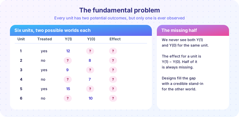
For each unit i and a binary treatment Di:
Yi(1)is the outcome ifDi = 1,Yi(0)is the outcome ifDi = 0,- the individual effect is
τi = Yi(1) − Yi(0), - the observed outcome is
Yi = Di Yi(1) + (1 − Di) Yi(0).
Only one of the two potential outcomes is revealed for each unit; the other is the counterfactual. This is the fundamental problem of causal inference (Holland, 1986). Causal inference is therefore a missing-data problem. We cannot learn τi, but we can try to learn averages of τi:
- ATE (average treatment effect):
E[Yi(1) − Yi(0)], the effect for a randomly chosen member of the population. - ATT (effect on the treated):
E[Yi(1) − Yi(0) | Di = 1], the effect for those who actually got the treatment.
The framework carries an assumption so quiet that it is easy to miss: SUTVA (stable unit treatment value assumption). It requires that one unit's treatment does not change another unit's outcome (no spillovers), and that there is a single, well-defined version of the treatment. A tutoring program that also improves a classmate's grades, or a vaccine that protects neighbours, violates the first; "job training" that means different things in different offices violates the second.
Why randomization works
Recall the decomposition from the overview: a naive comparison equals the ATT plus selection bias, E[Y(0) | D = 1] − E[Y(0) | D = 0]. If treatment is assigned by a coin flip, then D is independent of (Y(1), Y(0)), so E[Y(0) | D = 1] = E[Y(0) | D = 0] and the bias is zero. Therefore
E[Y | D = 1] − E[Y | D = 0] = E[Y(1) − Y(0)] = ATE
Randomization does not make individuals alike; it makes the groups alike in expectation on every characteristic, observed or unobserved. The difference in sample means is unbiased for the ATE, and equals the OLS slope in a regression of Y on D.
Analysing a trial
- Check balance. Compare pre-treatment variables across arms (a "Table 1"). Large standardized differences suggest a problem with the randomization or a small sample. A few significant differences among many variables occur by chance.
- Estimate the effect. Regress
YonDwith robust (HC) standard errors. The coefficient onDis the estimated ATE. - Adjust for covariates to gain precision. Adding pre-treatment covariates
Xthat predictY(especially the baseline value of the outcome) reduces residual variance and tightens the interval, without introducing bias, becauseXis unrelated toDby design. Never adjust for post-treatment variables, which can be affected by the treatment and create bias. - Report effect sizes and intervals, not just p-values. An effect is also best judged relative to what matters in practice.
Other design points: stratified (blocked) randomization guarantees balance on key variables; clustered randomization (assigning whole schools or villages) calls for cluster-robust standard errors; attrition (participants who drop out) can reintroduce selection if it differs by arm; and external validity (does the effect carry over to other settings?) is a separate question from internal validity.
Press Run (or Ctrl + Enter) to see the result here.
Program input · what you'd type while the program runs
Type the answers before you press Run, one per line. Each time the program reads a line (with input()), it gets the next line from this box.
Both estimates should be near 3.0. The adjusted standard error is smaller because the baseline score explains a lot of the variation in y; the point estimate barely moves, which is the sign of a well-randomized trial.
Power: how big a trial do you need?
A trial that is too small cannot detect a real effect. Power is the probability of rejecting a false null. It rises with the sample size and with the size of the effect relative to the noise.
Press Run (or Ctrl + Enter) to see the result here.
Program input · what you'd type while the program runs
Type the answers before you press Run, one per line. Each time the program reads a line (with input()), it gets the next line from this box.
For an effect of 0.2 standard deviations, about 800 participants in total are needed to reach 80% power; for 0.5 standard deviations, about 130. These magnitudes explain why many early studies of modest effects were underpowered.
Noncompliance: ITT and LATE
In practice not everyone follows their assignment: some assigned to a training program never show up, and some control individuals find a way in. Let Zi be the random assignment and Di the treatment actually received.
- The intention-to-treat (ITT) effect compares groups by assignment, regardless of what they did:
E[Y | Z = 1] − E[Y | Z = 0]. It is unbiased for the effect of the offer and it is what a policy that offers a program would produce. - Comparing those who took the treatment with those who did not (an "as-treated" or "per-protocol" comparison) throws away the randomization, because take-up is selective.
- Because
Zis random, it is a valid instrument forD(chapter 6). The Wald ratioITT / (share who comply)gives the LATE, the effect for compliers. With one-sided noncompliance (only the assigned can get treatment) the LATE equals the effect on the treated.
Press Run (or Ctrl + Enter) to see the result here.
Program input · what you'd type while the program runs
Type the answers before you press Run, one per line. Each time the program reads a line (with input()), it gets the next line from this box.
The ITT is about 3 times the compliance rate. Dividing by the take-up rate gives the effect for compliers, close to 3.0, while the as-treated comparison is badly biased upward.
When can't we randomize?
Experiments can be too expensive, unethical, or impossible: you cannot randomly assign countries to wars. Then researchers look for natural experiments, situations where nature or policy creates something close to random assignment, and for quasi-experimental designs that rely on explicit assumptions. The next two lessons cover the two most common ones.
Common misconceptions
"Randomization guarantees balance in every sample." It guarantees balance in expectation; any single trial can have imbalances, especially when small.
"Controlling for covariates in an RCT is cheating." Adjusting for pre-treatment covariates improves precision. Adjusting for post-treatment variables is what causes trouble.
"Per-protocol analysis is more honest than ITT." Comparing only compliers breaks the randomization; ITT preserves it.
"The ATE is what everybody experiences." It is an average; individual effects can differ widely.
Check your understanding
Quick check · 5 questions
of 5 answered You scored / 5 · perfect!
-
1. The ATT is the average effect for...
ATT = E[Y(1) - Y(0) | D = 1]. -
2. A coin-flip assignment makes the treatment independent of...
Independence from (Y(1), Y(0)) removes selection bias. -
3. Which variable should NOT be used as a control when analysing a randomized trial?
Post-treatment variables can be outcomes of the treatment and induce bias when controlled for. -
4. The ITT effect is 1.2 and 60% of those assigned to treatment take it up (no one in the control group does). The LATE is...
LATE = ITT / take-up = 1.2 / 0.6 = 2.0. -
5. SUTVA would be violated if...
A spillover to another unit means one unit's treatment affects another's outcome.
Summary
- Potential outcomes
Y(1)andY(0)define causal effects; only one is observed per unit, so we estimate averages (ATE, ATT). - A naive comparison equals the ATT plus selection bias; randomization makes the bias zero.
- Analyse trials with balance checks, a simple (robust) regression and pre-treatment covariates for precision; plan sample size with power.
- With noncompliance, ITT estimates the effect of the offer, and ITT divided by take-up estimates the LATE.
Track your progress
Create a free account to tick off lessons and pick up where you left off on any device.
of Econometrics lessons completed