


















Lesson 46 of 49 · Projects and Practice
Advanced practice problems
Fourteen problems covering heteroskedasticity, autocorrelation, instruments, panels, time series and causal designs, with worked answers and a Python checker.
You learn econometrics by doing it. These fourteen problems revisit chapters 5 to 8, mixing short calculations with questions about which method fits which situation. Try each one on paper first, then check your reasoning against the answers further down. Two code cells help you verify the numbers and explore further.
Do not rush to the answers. The most valuable part of a problem is the five minutes you spend stuck on it.
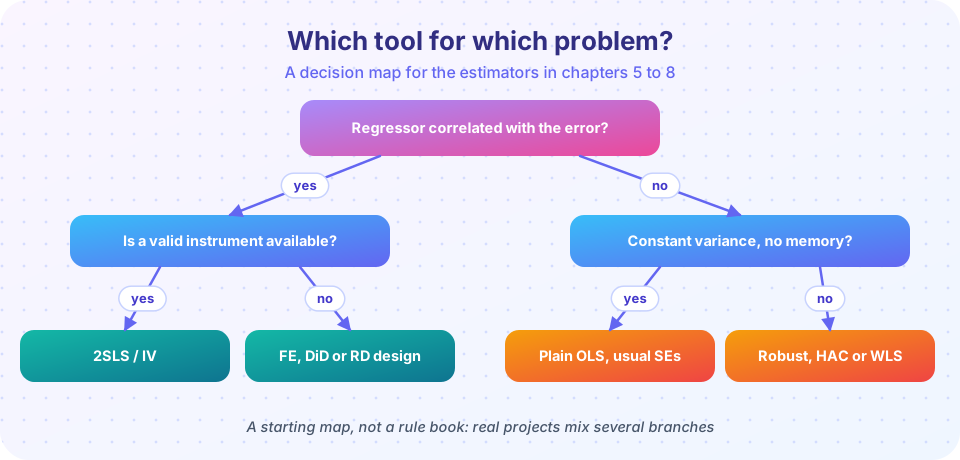
What you will learn
- How to decide which estimator or test a situation calls for.
- How to carry out the standard calculations by hand.
- How to check your work with short simulations.
Key terms
LM statistic: n × R² of an auxiliary regression. Wald ratio: the reduced-form change divided by the first-stage change. Half-life: the number of periods needed to close half of a gap. DiD: the change in the treated group minus the change in the control group. Fuzzy RD: the outcome jump divided by the treatment-probability jump.
Heteroskedasticity and autocorrelation
Problem 1. A Breusch-Pagan regression of squared residuals on 3 regressors, in a sample of 200, has R² = 0.06. Compute the LM statistic. The 5% critical value of a chi-square with 3 degrees of freedom is 7.81. What do you conclude?
Problem 2. After a Breusch-Pagan test rejects, a colleague says "your coefficients are now unreliable". Respond in two sentences.
Problem 3. In a time-series regression with strictly exogenous regressors and a large sample, d = 1.2. Estimate the first-order autocorrelation of the residuals and say what happens to the usual standard errors.
Problem 4. The error variance is Var(u | x) = σ² x with x > 0, and you want a WLS estimator of y = β0 + β1 x + u. What weights do you use, and what is the transformed equation?
Endogeneity and instruments
Problem 5. The true return to schooling is 0.08. Ability has an effect β2 = 0.2 on log wage, and in the data the regression of ability on schooling has slope δ1 = 0.3. What does OLS on schooling alone converge to?
Problem 6. A regressor is measured with classical error; its reliability ratio is 0.7 and the true slope is 0.5. What does OLS converge to?
Problem 7. A binary instrument Z is randomly assigned. Mean log wage is 10.8 when Z = 1 and 10.2 when Z = 0. Mean schooling is 13.1 when Z = 1 and 12.6 when Z = 0. Compute the IV (Wald) estimate of the return to schooling.
Problem 8. A model has 2 endogenous regressors and 5 excluded instruments. How many degrees of freedom does the Sargan test have? What does a rejection imply, and what does non-rejection not imply?
Panels and time series
Problem 9. In a firm panel, the Hausman test strongly rejects the random-effects specification. Which estimator would you report, and why? Name one variable you can no longer estimate with it.
Problem 10. An ADF test with a constant on the log of a country's price level gives a t statistic of −1.9 (5% critical value −2.86). What do you conclude and what do you do next?
Problem 11. An error correction model has speed of adjustment α = −0.25. If last period's gap was 8 units, what do you expect the gap's contribution to this period's change to be? After how many periods (to one decimal place) is half of an initial gap closed, assuming no further shocks?
Causal designs
Problem 12. A program is introduced in one region. Average outcomes: treated region 20 before and 26 after; control region 18 before and 21 after. Compute the DiD estimate and state the assumption it needs.
Problem 13. In a fuzzy RD, the outcome jumps by 1.5 at the cutoff and the probability of treatment jumps from 0.2 to 0.7. What is the estimated effect and for whom?
Problem 14. A randomized trial wants 80% power for a 5% two-sided test to detect an effect of 0.5 standard deviations, with equal group sizes. Roughly how many people are needed in each group?
Checking some answers in code
The cell below verifies the arithmetic of problems 1, 3, 5, 6, 7, 11, 12, 13 and 14. Try to predict each number first.
Press Run (or Ctrl + Enter) to see the result here.
Program input · what you'd type while the program runs
Type the answers before you press Run, one per line. Each time the program reads a line (with input()), it gets the next line from this box.
A small Monte Carlo to try yourself
This starter code estimates how often a 95% confidence interval for a slope covers the truth, with usual, HC0 and HC3 standard errors, as the sample grows from 20 to 200 observations and the error variance is uneven. Predict what the three curves will look like before you run it, then change the sample sizes or the strength of the heteroskedasticity and see what happens.
Press Run (or Ctrl + Enter) to see the result here.
Program input · what you'd type while the program runs
Type the answers before you press Run, one per line. Each time the program reads a line (with input()), it gets the next line from this box.
After running it: the usual interval stays far below 95% even in large samples, HC0 improves only slowly with n, and HC3 is close to the target from small samples on.
Answers
1. LM = 200 × 0.06 = 12 > 7.81: reject constant variance. Use robust standard errors (or model the variance).
2. A rejection concerns the variance of the errors. The coefficients stay unbiased under the usual exogeneity assumption; what is unreliable are the usual standard errors, which you repair with robust ones.
3. d ≈ 2(1 − ρ̂), so ρ̂ ≈ 0.4: positive autocorrelation. The coefficients remain unbiased, but the usual standard errors are typically too small, so use Newey-West (HAC) errors.
4. Weights w = 1/x. Divide the equation by √x: y/√x = β0 (1/√x) + β1 √x + u/√x. The transformed error has constant variance σ². (Note: there is no separate intercept column; the former constant is now 1/√x.)
5. plim b = β1 + β2 δ1 = 0.08 + 0.2 × 0.3 = 0.14, an upward bias of 0.06.
6. 0.7 × 0.5 = 0.35, attenuated toward zero.
7. (10.8 − 10.2) / (13.1 − 12.6) = 0.6 / 0.5 = 1.2. (The unrealistic size, 120% per year, is a sign the numbers are for practice only.)
8. 5 − 2 = 3 degrees of freedom. A rejection means the instruments do not all agree: at least one is probably invalid (or the model is misspecified). Non-rejection does not show validity: if all instruments share the same flaw, they agree, and the test passes.
9. Fixed effects: rejection says the unit effects are correlated with the regressors, so RE is inconsistent. FE cannot estimate time-invariant variables such as the firm's industry or founding year.
10. −1.9 > −2.86, so you cannot reject a unit root. Plot the series, check the first difference with the same test and, if it is stationary, model changes (log differences, i.e. inflation) or test for cointegration with other I(1) series. Remember the test has low power.
11. Contribution α × gap = −0.25 × 8 = −2 (the gap shrinks by 2). After h periods a fraction 0.75ʰ of the gap remains, so half-life = ln(0.5)/ln(0.75) ≈ 2.4 periods.
12. (26 − 20) − (21 − 18) = 6 − 3 = 3. Needs parallel trends: without the program, the treated region would have risen by 3 as the control did.
13. 1.5 / (0.7 − 0.2) = 3.0: the local effect for compliers at the cutoff (those whose treatment status changes because they cross it).
14. n ≈ 2 (1.96 + 0.84)² / 0.5² ≈ 63 per group, about 126 in total.
Check your understanding
Quick check · 5 questions
of 5 answered You scored / 5 · perfect!
-
1. Your regression uses quarterly data and the residuals show long runs of the same sign. Which standard errors do you report?
Runs of same-sign residuals indicate positive autocorrelation; HAC errors repair inference. -
2. A regressor is correlated with the error and you have a credible instrument. Which method fits?
Endogeneity calls for instrumental variables; the other tools fix variance problems. -
3. Firms observed for 10 years, unobserved firm quality correlated with advertising. Which model?
FE removes the unit effect even when it is correlated with the regressors. -
4. Two I(1) series with a stationary residual from their levels regression are...
A stationary linear combination of I(1) series is the definition of cointegration. -
5. A threshold rule assigns a benefit at a test score of 60. Which design?
Units just above and below the cutoff are compared.
Summary
- Match the tool to the problem: variance problems call for robust or modelled errors; endogeneity calls for instruments or designs; unobserved unit traits call for fixed effects; trending series call for unit-root and cointegration analysis.
- Carry out the standard calculations (LM, Wald, DiD, half-life, fuzzy RD, power) by hand and check them with code.
- Predict a simulation's outcome before running it.
Next: Glossary
Track your progress
Create a free account to tick off lessons and pick up where you left off on any device.
of Econometrics lessons completed