


















Lesson 25 of 49 · Violations: Heteroskedasticity and Autocorrelation
Testing for heteroskedasticity
Learn the Breusch-Pagan and White tests step by step, compute them by hand in Python, and see what a rejection does and does not mean.
A residual plot is the best first look, but a picture is a matter of opinion. One analyst sees a funnel; another sees noise. Formal tests give a common yardstick: they ask whether the pattern in the squared residuals is bigger than what chance alone would produce under constant variance.
Almost every heteroskedasticity test follows one idea. If the error variance depends on the regressors, then the squared residuals, our rough stand-in for the unobservable error variance, should be predictable from the regressors. So we regress the squared residuals on something and ask whether that auxiliary regression explains a significant share of their variation. This lesson builds the two most used tests, Breusch-Pagan and White, and gives you the judgement to use them.
What you will learn
- The null and alternative hypotheses of the Breusch-Pagan and White tests.
- How to compute the LM statistic
n × R²by hand and find its p-value. - Why White's test is more general but uses up more degrees of freedom.
- How to read a rejection, and why these tests are not a final answer.
Key terms
Auxiliary regression: a second regression run only to compute a test statistic. LM statistic: Lagrange multiplier statistic, here n × R² from the auxiliary regression. Chi-square distribution: the reference distribution for LM statistics; its degrees of freedom equal the number of slope terms in the auxiliary regression. Null hypothesis (H0): here, homoskedasticity. Power: the probability of rejecting H0 when it is false.
The Breusch-Pagan test
Take the model y = β0 + β1x1 + ... + βkxk + u and suppose the error variance may depend on the same regressors (or on any variables z you suspect):
Var(u | x) = σ² h(δ0 + δ1x1 + ... + δkxk)
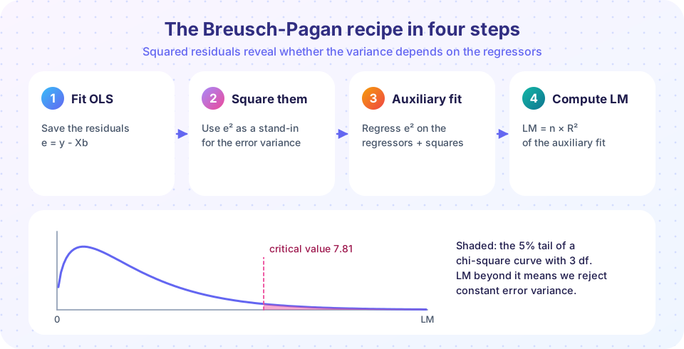
Homoskedasticity means δ1 = ... = δk = 0. The recipe uses only the residuals, so it needs no knowledge of the function h:
- Estimate the original model by OLS and save the residuals
e. - Square them:
e². - Regress
e²on the regressors (or on your chosenzvariables), with an intercept. Record the R² of this regression, writtenR²_aux. - Compute
LM = n × R²_aux. Under H0 and in large samples, LM follows a chi-square distribution withkdegrees of freedom, wherekis the number of slope terms in the auxiliary regression. - Reject constant variance when LM exceeds the chi-square critical value, equivalently when the p-value is below your significance level.
This is the studentized (Koenker) version, which does not require normal errors and is what most software reports by default. The original Breusch-Pagan statistic scales differently and relies on normality, which is a strong assumption you rarely want.
Notice the logic: if x tells you nothing about e², then R²_aux is close to zero, LM is small, and we keep H0. If the squared residuals rise steadily with x, R²_aux is noticeably positive and LM is large.
The White test
Breusch-Pagan detects variance that is a linear function of the regressors. What if the variance is U-shaped, or depends on an interaction? Halbert White (1980) proposed regressing e² on the regressors, their squares and their cross-products. With two regressors the auxiliary regression contains x1, x2, x1², x2², x1x2: five terms, so the test has 5 degrees of freedom. The general count is k(k + 3)/2 terms for k regressors (excluding dummies, whose squares duplicate themselves).
The flexibility has a price. Each added term costs a degree of freedom and reduces power, and with many regressors the auxiliary regression becomes huge. A common compromise is the special-case White test: regress e² on the fitted values ŷ and ŷ² only. That always uses 2 degrees of freedom, however many regressors you have, and captures the typical pattern "variance depends on the level of y".
A third classic is the Goldfeld-Quandt test, which sorts the data by a suspect variable, drops a middle chunk and compares the residual variance of the low and high groups with an F ratio. It is easy to explain and works when one variable drives the variance, but it is less general than the LM tests.
Computing it by hand
The code below implements the studentized Breusch-Pagan test and the special-case White test from scratch with numpy and scipy, on two invented datasets: one with constant variance and one with a funnel.
Press Run (or Ctrl + Enter) to see the result here.
Program input · what you'd type while the program runs
Type the answers before you press Run, one per line. Each time the program reads a line (with input()), it gets the next line from this box.
You should see small LM values and large p-values for the constant-variance data, and large LM values with tiny p-values for the funnel. Because the data are random, the exact numbers depend on the seed, but the contrast should be clear.
Looking at the distribution of the statistic
To see why a large n × R² is rare under H0, simulate many datasets with constant variance, compute LM each time and compare the histogram with the chi-square curve.
Press Run (or Ctrl + Enter) to see the result here.
Program input · what you'd type while the program runs
Type the answers before you press Run, one per line. Each time the program reads a line (with input()), it gets the next line from this box.
If the test is well behaved, about 5% of simulated statistics should land in the shaded tail. That is exactly what "5% significance level" promises.
Reading a rejection
A rejection tells you the squared residuals are related to the variables you used. It does not tell you the form of the variance, how large the problem is, or whether you should worry. In small samples these tests have limited power: a funnel can exist without a significant test. In large samples the opposite happens: tiny, harmless variation becomes "significant". A sensible protocol:
- Look at the residual plot first and judge the size of the problem.
- Run Breusch-Pagan, and the White test if you suspect non-linear dependence.
- Whatever the test says, report robust standard errors as a default for cross-section data. If the test fails to reject and robust and usual errors are nearly identical, nothing is lost.
A common error is pre-testing: using the test to decide whether to correct. Because tests err, it is safer to always correct. The cost of robust errors when the variance is in fact constant is small in moderate samples; the cost of ignoring uneven variance can be large.
Also remember that an apparent failure may point at the model. If a log transformation of y makes the funnel vanish, the real lesson was about functional form (see chapter 4 on specification).
Common misconceptions
"A non-significant Breusch-Pagan test proves homoskedasticity." Failing to reject is not proof. The test may simply lack power, especially in small samples or with the wrong choice of auxiliary variables.
"A significant test means I must switch to WLS." A rejection justifies repairing inference. Robust standard errors do that without any model for the variance. WLS needs you to know or estimate the form.
"The LM statistic is a t statistic." It follows a chi-square distribution and tests all auxiliary slopes jointly.
Check your understanding
Quick check · 5 questions
of 5 answered You scored / 5 · perfect!
-
1. In the Breusch-Pagan test, what is regressed on the regressors?
The squared residuals stand in for the error variance. If they can be predicted from the regressors, the variance is not constant. -
2. With an auxiliary R-squared of 0.04 and n = 250, what is the LM statistic?
LM = n x R-squared = 250 x 0.04 = 10. -
3. A White test has two regressors and includes all squares and cross-products. How many auxiliary terms (degrees of freedom) does it have?
x1, x2, x1 squared, x2 squared and x1 times x2 give 5 terms, which matches k(k+3)/2 with k = 2. -
4. Why is the special-case White test (e-squared on fitted values and their square) convenient?
Using the fitted value and its square uses only two auxiliary slopes, which preserves power in models with many regressors. -
5. Which is the best practical advice after a Breusch-Pagan test that fails to reject?
A failure to reject is not proof of constant variance, and robust errors cost little, so they are a sound default.
Summary
- Heteroskedasticity tests regress squared residuals on regressors (Breusch-Pagan), or on regressors, squares and cross-products (White).
- The LM statistic
n × R²_auxis compared with a chi-square distribution; the degrees of freedom equal the number of auxiliary slopes. - Rejections do not reveal the form of the variance, and non-rejections are not proof of constancy.
- Plot first, test second, and report robust standard errors as a safe default.
Track your progress
Create a free account to tick off lessons and pick up where you left off on any device.
of Econometrics lessons completed