


















Lesson 8 of 49 · Data and the Regression Idea
The conditional expectation function
Understand the conditional expectation function, the law of iterated expectations, why E[y|x] is the best predictor and how linear regression approximates it, with runnable examples.
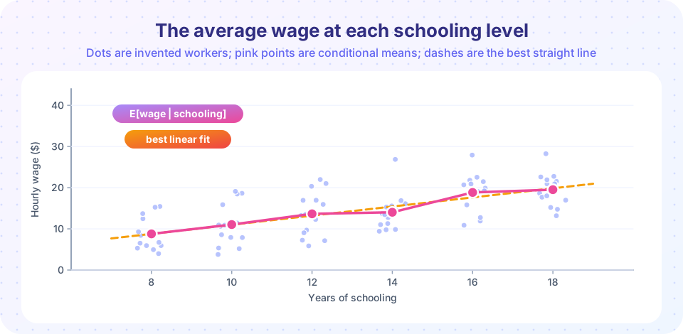
Suppose someone asks you to guess the hourly wage of a stranger. With no other information, your best guess is the average wage in the population. Now you learn the stranger has 16 years of schooling. You would revise your guess to the average wage among people with 16 years of schooling. That revised guess is a conditional expectation, and the rule that gives it for every level of schooling is the conditional expectation function, or CEF.
The CEF is the central object of regression analysis. Regression is, in the end, a method for estimating it. This lesson makes the idea precise and shows why it deserves its starring role.
What you will learn
- The definition of
E[y | x]and how to read it. - The decomposition
y = E[y | x] + εand what the errorεmeans. - The law of iterated expectations.
- Why the CEF is the best predictor of
y, and how linear regression approximates it.
Key terms
Conditional expectation, E[y | x]: the average of y among all units that share the value x.
CEF: the function m(x) = E[y | x] that gives that average for every x.
Law of iterated expectations (LIE): E[y] = E[ E[y | x] ], the overall average equals the average of the group averages.
Mean squared error (MSE): the average squared difference between a prediction and the outcome.
Best linear predictor: the straight line that minimizes the MSE among all lines.
Definition and a worked example
For a discrete x, the conditional expectation at the value x = a is the average of y over only the population with x = a. Suppose the working population consists of three schooling groups:
Schooling x |
Share of workers | Average wage E[wage | x] |
|---|---|---|
| 12 years | 50% | $16 |
| 16 years | 30% | $22 |
| 18 years | 20% | $26 |
Then E[wage | educ = 16] = 22: the CEF at 16 years of schooling. The CEF is the whole column of conditional averages, a function from schooling to expected wage. It has nothing to do with whether any single person fits it; it describes averages over groups.
Notice the notation E[y | x] is itself a function of x, hence random if x is random. This subtlety makes the next result work.
The law of iterated expectations
If you average the group averages, weighting by group shares, you recover the overall average. In the table:
E[wage] = 0.5 × 16 + 0.3 × 22 + 0.2 × 26 = 8 + 6.6 + 5.2 = 19.8
This is the law of iterated expectations: E[y] = E[ E[y | x] ]. It seems obvious once seen. It is used repeatedly in proofs, for instance to show that regression estimates are unbiased (Chapter 4). A related fact, the law of total variance, splits the variance of y into the part explained by x (the variance of the CEF) and the part left over (the average conditional variance). That is exactly what the R-squared statistic measures, in Chapter 3.
The decomposition: signal plus noise
Define the deviation of each person from their group average:
ε = y − E[y | x] so that y = E[y | x] + ε
The first part is the systematic part, explained by x. The second, ε, is the unexplained part. Two properties hold by construction, not by assumption:
E[ε | x] = 0. Within every group, deviations from the group average cancel out, because that is what an average does.εis uncorrelated with any function ofx.
These are properties of how we defined ε. They do not mean that ε is "pure luck unrelated to causes". In the wage example ε contains ability, and ability is part of why some workers in the 16-year group earn more than others. Whether ε also contains something that causes both schooling and wages is a different, harder question about causality, addressed from Chapter 4 on.
Why the CEF is the best predictor
Say you want a rule g(x) that predicts y as accurately as possible, where "accurate" means a small mean squared error E[(y − g(x))²]. It turns out that the best rule is the CEF. The idea of the proof is short. Add and subtract m(x) = E[y | x] inside the square:
E[(y − g)²] = E[(y − m)²] + E[(m − g)²] + 2·E[(y − m)(m − g)]
The cross term is zero because y − m = ε has conditional mean zero while m − g depends only on x. What remains is E[(y − m)²], which does not depend on g, plus E[(m − g)²], which is never negative and is smallest, namely zero, when g = m. So no other function of x beats the CEF in mean squared error.
In words: the CEF is the best you can do with x alone, and what you cannot predict, the ε, is irreducible noise relative to that information.
From the CEF to regression
The CEF can be any shape: a straight line, a curve, even a staircase. We usually cannot know it without enormous data, so we approximate it. A linear regression picks the straight line that minimizes the mean squared error among all lines:
b1 = Cov(x, y) / Var(x), b0 = E[y] − b1 · E[x]
Two facts connect this line to the CEF.
- If the CEF is linear, the best linear predictor is the CEF. Regression then estimates it without distortion.
- If the CEF is not linear, the regression line is still the best linear approximation to the CEF in the mean squared error sense: it is the line closest to the pink points in the picture, weighted by how many workers sit at each
x.
That second fact is liberating. A straight line is almost never literally true, yet it remains a useful, well-defined summary of how the average outcome changes with x. You may then add squares or logs to let the fit bend (Chapter 3).
A caution about causation
The CEF answers "among people who have x = a, what is the average of y?" It does not answer "what would happen to this person's y if we changed x to a?" The workers with 18 years of schooling earn more on average than those with 12, but they also differ in other ways. The CEF is a statement about description and prediction; interpreting its slope as a causal effect requires extra assumptions.
Many regressors
Nothing changes when x is a collection of variables (x1, x2, ..., xk): the CEF E[y | x1, ..., xk] is the average of y among units with those exact values. This is hard to estimate when k is large because each combination of values has few observations (the "curse of dimensionality"), which is another reason we turn to parametric approximations such as a linear equation.
Common misconceptions
"The CEF tells me what happens to a person if I change x." It describes averages across groups that already differ. Causal reading needs more.
"Regression requires the true relationship to be a straight line." Regression estimates the best linear approximation to the CEF whatever its shape. The estimate can still be informative, though it may mislead at the extremes.
"The error term ε is whatever I forgot, so it is independent of everything." By construction ε has conditional mean zero given x, but that does not rule out that ε moves with other things, such as a variable I left out.
Try it
First example: compute the CEF by group averaging on a large simulated sample, and verify the law of iterated expectations numerically. The numbers are invented, with group averages near 16, 22 and 26.
Press Run (or Ctrl + Enter) to see the result here.
Program input · what you'd type while the program runs
Type the answers before you press Run, one per line. Each time the program reads a line (with input()), it gets the next line from this box.
Second example: a prediction contest. Because the simulated CEF is a curve, three predictors are compared by mean squared error: the overall mean, the best straight line and the true CEF (group averages). The CEF should win, and its error should be close to the noise variance, 9, which no predictor using x alone can beat.
Press Run (or Ctrl + Enter) to see the result here.
Program input · what you'd type while the program runs
Type the answers before you press Run, one per line. Each time the program reads a line (with input()), it gets the next line from this box.
Third example: draw the CEF and the best line together for the curved case, and see where the line misses the averages.
Press Run (or Ctrl + Enter) to see the result here.
Program input · what you'd type while the program runs
Type the answers before you press Run, one per line. Each time the program reads a line (with input()), it gets the next line from this box.
Check your understanding
Quick check · 5 questions
of 5 answered You scored / 5 · perfect!
-
1. In the table of three schooling groups, what is E[wage | educ = 18]?
The conditional expectation at educ = 18 is the average wage in that group, $26. -
2. The law of iterated expectations says that
E[y] = E[E[y | x]]: weight each group's average by the group's share and add up. -
3. Among all functions of x, which minimizes the mean squared prediction error of y?
The CEF is the best predictor; the best linear predictor is the best among lines only. -
4. If the CEF is not linear, what does the regression line estimate?
OLS targets the line closest to the CEF in mean squared error, even when the CEF bends. -
5. Which is true of ε = y − E[y | x] by construction?
Deviations from a group's average cancel within the group, so the conditional mean of ε is zero.
Summary
E[y | x]is the average ofyamong units with the givenx; the whole function is the CEF.y = E[y | x] + ε, whereE[ε | x] = 0by construction.- The law of iterated expectations:
E[y] = E[E[y | x]]. - The CEF is the best predictor of
ygivenxin mean squared error. - Linear regression estimates the best linear approximation to the CEF; its causal reading needs extra assumptions.
Track your progress
Create a free account to tick off lessons and pick up where you left off on any device.
of Econometrics lessons completed