


















Lesson 15 of 49 · Simple and Multiple Regression
Functional forms, logs and dummies
Learn how to model percentage effects with logs, curves with quadratics and group differences with dummies and interactions, and how to interpret each correctly in OLS.
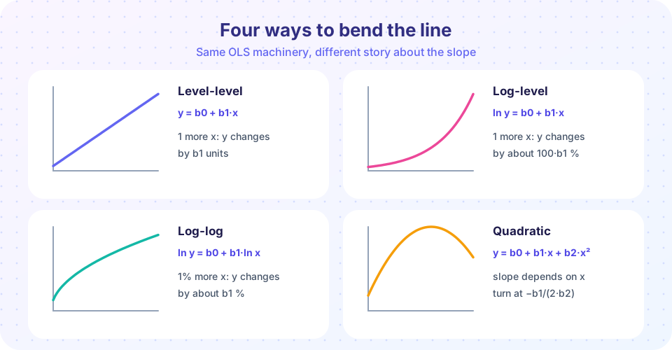
"Linear regression" sounds restrictive: does it only fit straight lines? No. The word linear refers to how the coefficients enter the equation, not to the shape of the relationship in the original variables. By transforming variables (taking logs, squaring them, creating dummies) you can model percentage changes, diminishing returns, thresholds and differences between groups, all with the same OLS machinery and the same estimation formulas.
This lesson covers the four tools you will use most: logarithms, quadratics, dummy variables and interactions. For each one the key skill is interpretation: saying in words what a coefficient means.
What you will learn
- What makes a model "linear" and why transformed variables are allowed.
- How to interpret level-level, log-level, level-log and log-log models.
- How to model curvature with a quadratic and find a turning point.
- How dummy variables and interactions represent group differences, and how to avoid the dummy trap.
Key terms
Natural logarithm, ln: the logarithm to base e ≈ 2.718; ln(y) changes by about 0.01 when y rises by about 1%.
Elasticity: the percentage change in y per 1% change in x.
Dummy variable: a 0/1 indicator for membership in a group.
Reference (base) category: the group left out of a set of dummies; others are compared with it.
Interaction: a product of two variables that lets the effect of one depend on the other.
Linear in parameters
A model is linear in parameters if it can be written y = β0 + β1·f1(x) + β2·f2(x) + ..., where the f are known functions of the data. So wage = β0 + β1·educ + β2·educ² is linear in the βs even though it is a parabola in educ: define x2 = educ² as a new variable and you have an ordinary multiple regression. By contrast y = β0 + x^β1 is not linear in parameters and needs nonlinear estimation.
Logarithms
The natural logarithm is the economist's favorite transformation, for three reasons: many economic variables (wages, prices, GDP) are right-skewed and nearly symmetric in logs; effects are often proportional (a 10% raise matters equally to a low and a high earner); and coefficients on logs read as percentages.
The key approximation: for small changes, Δ ln(y) ≈ Δy / y, the proportional change. A change of 0.05 in ln(y) is about a 5% change in y.
| Model | Equation | Reading the slope β1 |
|---|---|---|
| Level-level | y = β0 + β1·x |
One more unit of x: y changes by β1 units |
| Log-level | ln y = β0 + β1·x |
One more unit of x: y changes by about 100·β1 percent |
| Level-log | y = β0 + β1·ln x |
A 1% rise in x: y changes by about β1/100 units |
| Log-log | ln y = β0 + β1·ln x |
A 1% rise in x: y changes by about β1 percent (an elasticity) |
Worked example: a log-level wage equation
Suppose a regression of ln(wage) on schooling gives ln(wage)-hat = 1.50 + 0.08·educ. The slope 0.08 means each extra year of schooling goes with about 8% higher wages. The exact percentage is 100 × (e^0.08 − 1) = 8.33%. The approximation is good for small coefficients and worsens for large ones: with β1 = 0.5 the approximation says 50% but the exact figure is 100 × (e^0.5 − 1) ≈ 64.9%.
Also note the intercept: 1.50 is the predicted log wage at zero schooling, so e^1.50 ≈ 4.48 dollars. One caution: predicting y from a log model by simply exponentiating the fitted log tends to underpredict the mean of y, because the exponential of an average is not the average of exponentials; a correction exists but is beyond this lesson.
Worked example: elasticity
In a log-log demand equation ln(quantity)-hat = 7.2 − 1.2·ln(price), the slope −1.2 is the price elasticity of demand: a 1% rise in price goes with about a 1.2% fall in the quantity demanded. Because the elasticity is the same at every price level, the log-log form is a convenient constant-elasticity model.
When not to take logs
Logs require positive values. If a variable can be zero or negative (profit, a net change), taking logs is impossible without ad-hoc fixes. And variables already measured in percentages or rates are usually left in levels; then you describe changes in percentage points. A rise in an unemployment rate from 5% to 7% is a two percentage-point rise but a 40% percent rise; mixing the two phrases is a classic error.
Quadratics: curves and turning points
Returns often diminish. Wages rise with experience at first, then flatten, and may fall. Add the square:
wage = β0 + β1·exper + β2·exper² + u
The effect of one more year of experience is no longer a single number. Differentiating, or reasoning with small changes, the marginal effect is
Δwage / Δexper ≈ β1 + 2·β2·exper
so it depends on the level of experience. With estimates b1 = 0.50 and b2 = −0.01:
- at
exper = 0, the marginal effect is0.50; - at
exper = 10, it is0.50 − 0.20 = 0.30; - the turning point is where the marginal effect is zero:
exper* = −b1 / (2·b2) = 0.50 / 0.02 = 25years.
After 25 years the fitted curve slopes down. Never interpret b1 alone as "the effect of experience"; it is only the slope at exper = 0. Check that the turning point falls inside the range of your data: a turning point at 80 years of experience is irrelevant, and a quadratic may behave wildly outside the sample.
Dummy variables
A dummy variable takes the value 1 if an observation belongs to a group and 0 otherwise. In wage = β0 + β1·female + u, with female = 1 for women:
β0is the average wage of men (female = 0);β0 + β1is the average wage of women;β1is the difference in average wages between women and men.
Regressing on a single dummy gives exactly the difference in group means. Add other variables and β1 becomes the difference holding them constant, for example wage = β0 + β1·female + β2·educ: the gap between a woman and a man with the same schooling. Geometrically, the dummy shifts the intercept: two parallel lines, one for each group.
Several categories and the dummy trap
For a variable with m categories (say four regions), create m − 1 dummies and leave one out as the reference category. Each coefficient is the difference between that region and the reference. Including all m dummies and the intercept is the dummy variable trap: the dummies add up to the intercept column, causing perfect collinearity. Equivalent alternatives are to drop the intercept (then each dummy coefficient is a group mean) or to choose a different reference category; the fitted values are identical, only the meaning of the coefficients changes.
Interactions
What if the slope differs between groups? Add an interaction term, the product of the dummy and the continuous variable:
wage = β0 + β1·female + β2·educ + β3·(female × educ) + u
For men the slope on educ is β2. For women it is β2 + β3, so β3 is the difference in the return to schooling between women and men. The intercept differs by β1. Interactions let the effect of one variable depend on another, and they are the workhorse of heterogeneity analysis.
Common misconceptions
"A log-level coefficient of 0.08 means wages rise by 0.08." It means about 8%, because the dependent variable is in logs.
"Percent and percentage points are interchangeable." A rate moving from 5% to 7% is up 2 percentage points and up 40 percent.
"The coefficient on experience in a quadratic is the effect of experience." It is only the slope at zero experience. Use b1 + 2·b2·exper.
"A dummy coefficient is the group's average." It is the difference from the reference group (given the other regressors).
Try it
First example: simulate a log-wage equation, estimate it and convert the slope to an exact percentage. The data are invented, with a true slope of 0.08.
Press Run (or Ctrl + Enter) to see the result here.
Program input · what you'd type while the program runs
Type the answers before you press Run, one per line. Each time the program reads a line (with input()), it gets the next line from this box.
Second example: regress on a dummy and confirm that the coefficient equals the difference in group means. Then add schooling and see the gap change when we compare people with equal schooling.
Press Run (or Ctrl + Enter) to see the result here.
Program input · what you'd type while the program runs
Type the answers before you press Run, one per line. Each time the program reads a line (with input()), it gets the next line from this box.
Third example: fit a quadratic, compute the turning point and see it on a plot. The data are invented with a true turning point at 25 years of experience.
Press Run (or Ctrl + Enter) to see the result here.
Program input · what you'd type while the program runs
Type the answers before you press Run, one per line. Each time the program reads a line (with input()), it gets the next line from this box.
Check your understanding
Quick check · 5 questions
of 5 answered You scored / 5 · perfect!
-
1. In ln(wage) = 1.5 + 0.08·educ, the slope means
With the dependent variable in logs, 100 times the slope is the approximate percent change in the outcome. -
2. In ln(q) = 7.2 − 1.2·ln(p), a 1% rise in price goes with about
The log-log slope is an elasticity: the percent change in q per 1% change in p. -
3. With b1 = 0.50 and b2 = −0.01 in wage = b0 + b1·exper + b2·exper², the turning point is at
−b1/(2·b2) = −0.50/(−0.02) = 25. -
4. An unemployment rate rises from 5% to 7%. This is
The rise is 2 percentage points, which is 2/5 = 40 percent of the original rate. -
5. To include a four-category variable (with an intercept) you should
All four dummies plus the intercept cause perfect collinearity (the dummy trap).
Summary
- A regression is linear in parameters, so logs, squares and interactions are all allowed.
- Log-level slopes are about 100·β percent; log-log slopes are elasticities; take exact percentages with
100(e^β − 1)for large β. - In a quadratic the marginal effect is
β1 + 2β2·xand the turning point is−β1/(2β2). - A dummy coefficient is a group difference relative to the reference category; use
m − 1dummies formgroups. - Interactions let slopes differ between groups.
Next: Chapter 3 review
Track your progress
Create a free account to tick off lessons and pick up where you left off on any device.
of Econometrics lessons completed