


















Lesson 32 of 49 · Instrumental Variables and Endogeneity
Testing instruments: weak, invalid and unnecessary
Learn how to check an instrument: the first-stage F rule, why weak instruments bias IV, the Sargan and Hansen J tests, and the Hausman endogeneity test.
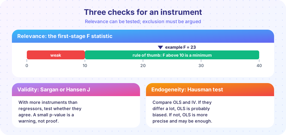
An instrument is a claim about the world, and claims need scrutiny. A careless IV analysis can be worse than OLS: a weak instrument gives an estimate that is both imprecise and biased, an invalid instrument gives a precise estimate of the wrong number, and an unnecessary IV analysis throws away precision when OLS would have been fine. Three families of checks guard against these three failures.
This lesson walks through them in the order a careful analyst would: strength first, validity second, necessity third. Remember throughout that no statistic can prove the exclusion restriction; tests can only reveal some ways in which it might fail.
What you will learn
- How to compute and read the first-stage F statistic, and why weak instruments cause bias.
- How the Sargan and Hansen J tests work for overidentified models, and what they cannot tell you.
- How to run the Durbin-Wu-Hausman test for endogeneity.
- A checklist for reporting an IV analysis.
Key terms
Weak instrument: an instrument with little explanatory power for the endogenous regressor in the first stage. First-stage F: the F statistic for the joint significance of the excluded instruments. Overidentifying restriction: an extra instrument beyond the number needed, which gives a testable implication. Sargan test / Hansen J: tests of whether all instruments are uncorrelated with the structural error. Hausman test: a test of whether OLS and IV give the same answer.
Check 1: is the instrument strong?
Recall β1_IV = Cov(z, y) / Cov(z, x). If the instrument barely moves x, the denominator is near zero. Two nasty things follow:
- The estimate becomes very noisy: dividing by a small, noisy number.
- Even a tiny correlation between
zand the error, harmless for a strong instrument, becomes a large bias. In the limit of a useless instrument,b_IVconverges toward the (biased) OLS estimate.
Bound, Jaeger and Baker (1995) showed that instruments with very small first-stage R² can give IV estimates almost as biased as OLS, for example in studies that used quarter of birth as an instrument for schooling with enormous samples, where the instrument was nonetheless weak.
The diagnostic. In the first stage, regress x on the controls and the excluded instruments, then test the joint hypothesis that all the instrument coefficients are zero. The F statistic is
F = [(RSSr − RSSu) / q] / [RSSu / (n − k)]
where q is the number of excluded instruments, RSSu the unrestricted residual sum of squares and RSSr the restricted one (without instruments). The rule of thumb from Staiger and Stock (1997) is F above 10. Stock and Yogo (2005) made this more precise with critical values for the maximum acceptable bias or size distortion; their values depend on the number of instruments and are larger than 10 when you have many instruments. With heteroskedasticity or clustering, use a robust version of the F statistic, such as the Kleibergen-Paap rk statistic or the effective F of Olea and Pflueger, and look for newer rules when your software provides them.
A modern remark: a first-stage F barely above 10 is not comfortable. Lee, McCrary, Moreira and Porter (2022) argued that when inference is based on the usual t-test, one needs F well above 10 (around 100 for a 5% test to be reliable). When F is small, use methods that are robust to weak instruments, such as the Anderson-Rubin confidence set, which stays valid at any strength.
What to do about weak instruments. Find a stronger instrument; use fewer, better instruments rather than many weak ones; use a limited-information maximum likelihood (LIML) estimator, which has better small-sample behaviour than 2SLS; or report weak-instrument-robust confidence sets.
Check 2: are the instruments valid?
Suppose you have more instruments than endogenous regressors: you are overidentified. Then the model contains an internal consistency check. If all instruments are valid, using different subsets of them should give similar estimates. If one instrument has a direct effect on y, the estimates diverge.
Sargan test. Estimate 2SLS and save the residuals û. Regress û on all exogenous variables (controls and all instruments). Then J = n R² of this regression follows approximately a chi-square distribution with degrees of freedom equal to the number of overidentifying restrictions (the number of excluded instruments minus the number of endogenous regressors). A large J rejects the joint validity of the instruments.
Hansen J. Hansen's version drops the homoskedasticity assumption and is the standard output after GMM or robust 2SLS. Interpret it the same way.
What the test does not tell you:
- It maintains that enough instruments are valid. If all instruments share the same flaw (for example, they are all correlated with ability in the same way), the estimates agree and the test passes, even though they are all wrong.
- It has low power against subtle violations.
- With a single instrument and a single endogenous regressor the model is just identified, and no test exists. Validity then rests entirely on argument.
A significant J does not say which instrument is bad. Examine each instrument's estimate separately and ask which is hardest to defend.
Check 3: is IV even needed? The Hausman test
IV costs precision. If the regressor is in fact exogenous, OLS is better. The Hausman test compares the OLS and IV estimates: under the null of exogeneity both are consistent and OLS is efficient, so their difference should be small. A convenient regression form (Durbin-Wu-Hausman):
- Run the first stage and save the residuals
v̂. - Add
v̂to the structural equation:y = β0 + β1x + γ'w + ρ v̂ + e, and estimate by OLS. - A t test of
ρ = 0is the test of exogeneity. Ifρis significantly different from zero,xis endogenous.
Why it works: v̂ captures the part of x that is not explained by the instrument. If that part is related to y after controlling for x, then the variation in x that is driven by hidden factors matters, which is endogeneity. Use a heteroskedasticity-robust t statistic in applications. Remember that the test needs valid instruments to be informative, and failing to reject does not prove exogeneity: with a weak instrument the test has little power.
All three checks in code
The simulation below has two instruments, a hidden confounder, and a true effect of 0.10. In the first run both instruments are valid. In the second, the second instrument also affects the outcome directly (a violation of exclusion).
Press Run (or Ctrl + Enter) to see the result here.
Program input · what you'd type while the program runs
Type the answers before you press Run, one per line. Each time the program reads a line (with input()), it gets the next line from this box.
In the valid case the F statistic is large, the IV estimate is near 0.10, J is unremarkable and the Hausman t statistic is large (OLS is biased, so IV is needed). In the second run, the direct effect pulls the IV estimate away from 0.10 and J rejects.
Weak instruments in action
Press Run (or Ctrl + Enter) to see the result here.
Program input · what you'd type while the program runs
Type the answers before you press Run, one per line. Each time the program reads a line (with input()), it gets the next line from this box.
As the instrument weakens, the histogram widens and the typical IV estimate drifts away from the true value (dashed line) toward the OLS value (pink line). That is the weak-instrument bias.
A reporting checklist
- State the instrument and give an argument for exclusion in plain words, ideally with institutional evidence.
- Report the first-stage coefficient and the first-stage F (robust if needed).
- Report the reduced form: if the instrument does not predict the outcome, be suspicious of any IV result.
- If overidentified, report Hansen J and discuss each instrument.
- Compare OLS and IV and say why they differ in the direction you expected.
- Be explicit about whose effect you estimated (LATE).
Common misconceptions
"F > 10 proves the instrument is valid." F measures strength only. Validity is separate.
"A passed J test means exclusion holds." J only checks agreement among instruments; if all share a flaw, the test passes.
"A weak instrument just makes standard errors big." It also makes the estimate biased toward OLS, and the usual t test misleading.
Check your understanding
Quick check · 5 questions
of 5 answered You scored / 5 · perfect!
-
1. The Staiger-Stock rule of thumb for instrument strength is...
An F statistic on the excluded instruments below about 10 flags a weak instrument. -
2. In a weak-instrument setting, the IV estimator tends to be biased toward...
With no first-stage strength, IV loses its advantage and converges toward the biased OLS value. -
3. You have 3 instruments and 1 endogenous regressor. How many degrees of freedom does the Sargan test have?
Overidentifying restrictions equal excluded instruments minus endogenous regressors: 3 - 1 = 2. -
4. The regression-based Hausman test adds which variable to the structural equation?
A significant coefficient on the first-stage residual indicates that x is endogenous. -
5. A single instrument for a single endogenous regressor. Which check is impossible?
The model is just identified, so there are no overidentifying restrictions to test.
Summary
- Strength: the first-stage F should be well above 10 (and robust to heteroskedasticity); weak instruments bias IV toward OLS.
- Validity: Sargan or Hansen J tests agreement among instruments, not the exclusion restriction itself; argue exclusion in words.
- Necessity: the Hausman test asks whether OLS and IV differ; failing to reject is weak evidence for exogeneity.
- Report the first stage, the reduced form, the comparison with OLS and the interpretation of the estimate.
Next: Chapter 6 review
Track your progress
Create a free account to tick off lessons and pick up where you left off on any device.
of Econometrics lessons completed