


















Lesson 27 of 49 · Violations: Heteroskedasticity and Autocorrelation
Serial correlation and HAC standard errors
Understand AR(1) errors, test for serial correlation with Durbin-Watson and Breusch-Godfrey, and repair inference with Newey-West HAC standard errors.
Economic time series have momentum. If the central bank surprises the market this quarter, the effect rarely vanishes by next quarter. If a harvest fails this year, prices stay elevated for a while. Whatever the regression leaves unexplained tends to inherit that persistence: the error term this period is related to the error term last period. The technical name is serial correlation or autocorrelation.
The classical assumption said errors in different observations are uncorrelated. When data are ordered in time, that is often false. This lesson explains what goes wrong, how to detect it with the Durbin-Watson and Breusch-Godfrey tests, and how to repair the standard errors with the Newey-West method.
What you will learn
- The AR(1) error model and its meaning.
- Why positive autocorrelation makes the usual standard errors too small.
- How to compute and interpret the Durbin-Watson statistic and the Breusch-Godfrey test.
- How the Newey-West HAC estimator works, and how to choose its lag length.
Key terms
AR(1) errors: ut = ρ ut−1 + εt, where εt is a well-behaved shock and |ρ| < 1. Autocorrelation function (ACF): correlations between a series and its own lags. Durbin-Watson statistic d: a summary of first-order residual correlation, between 0 and 4. HAC: heteroskedasticity and autocorrelation consistent covariance estimator. Bandwidth (lag truncation): how many lags of residual products the HAC estimator uses.
The AR(1) error model
The simplest model of persistence is
ut = ρ ut−1 + εt, with εt having mean zero, constant variance σε² and no correlation over time.
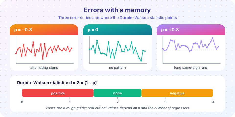
The parameter ρ is the correlation between neighbouring errors. When ρ > 0 shocks persist: positive errors tend to be followed by positive errors, producing long runs of residuals of the same sign. When ρ < 0 the errors zigzag. When ρ = 0 we are back in the classical world. The correlation h periods apart is ρʰ, so it decays geometrically.
Persistence also inflates the variance of the error: Var(ut) = σε² / (1 − ρ²). With ρ = 0.9 the error variance is more than five times the shock variance.
What serial correlation does
The same dichotomy as before applies. If the regressors are strictly exogenous, OLS remains unbiased and consistent, but the usual variance formula is wrong. Consider the sample mean of a persistent series: successive observations repeat each other's information, so the effective sample size is smaller than T. With ρ = 0.8, the mean of T = 100 observations behaves as if you had far fewer independent draws. Regression slopes inherit this loss when the regressors are also persistent, which most macro and finance variables are. The usual standard errors are then too small, t statistics inflated and spurious "significance" common.
A second, more serious problem arises when the regression contains a lagged dependent variable (yt−1 as a regressor) and the errors are serially correlated: yt−1 is then correlated with ut−1, which is correlated with ut, so OLS becomes biased and inconsistent. We treat this as a signal that the dynamics are misspecified, not as something to patch with standard errors.
Detecting it: plots and the autocorrelation function
Begin with a plot of residuals against time. Long same-sign runs mean positive autocorrelation; frequent sign flips mean negative. Then compute the sample correlation of et with et−1, and with a few more lags. In practice economists plot the ACF with approximate confidence bands at ±2/√T.
The Durbin-Watson test
James Durbin and Geoffrey Watson (1950, 1951) proposed
d = Σt=2..T (et − et−1)² / Σt=1..T et²
Expanding the square shows d ≈ 2(1 − ρ̂), where ρ̂ is the first-order residual correlation. So d near 2 means no first-order autocorrelation, near 0 means strong positive autocorrelation, near 4 means strong negative autocorrelation. Critical values depend on T and the number of regressors in a complicated way, so tables give a lower bound dL and an upper bound dU: below dL reject, above dU do not reject, between them the test is inconclusive. Modern software often computes an exact p-value instead.
The test has limits. It checks only first-order correlation, it requires strictly exogenous regressors (it is invalid with a lagged dependent variable, where d is biased toward 2), and it assumes a regression with an intercept.
The Breusch-Godfrey test
The Breusch-Godfrey test overcomes these limits. To test for autocorrelation up to order p:
- Fit the model by OLS and save residuals
et. - Regress
eton the original regressors and onet−1, ..., et−p(setting missing early lags to zero). - Compute
LM = n × R²of this auxiliary regression. - Under H0 of no autocorrelation,
LMis approximately chi-square withpdegrees of freedom.
Including the original regressors in step 2 is what makes the test valid even when a lagged dependent variable is among them. You can choose p to match the data frequency: 4 for quarterly series, 12 for monthly series, for example.
Newey-West HAC standard errors
If the test rejects, or if you simply expect persistence, repair the standard errors rather than trusting the usual ones. Whitney Newey and Kenneth West (1987) extended the sandwich idea. The meat of the sandwich now has to include cross-products of residuals at different dates:
S = Σt et² xt xt' + Σl=1..L wl Σt=l+1..T et et−l (xt xt−l' + xt−l xt')
with Bartlett weights wl = 1 − l/(L + 1), which shrink with the lag and guarantee a positive semi-definite estimate. The HAC covariance is (X'X)⁻¹ S (X'X)⁻¹. The statistic is consistent under both heteroskedasticity and autocorrelation of unknown form, provided L grows slowly with T.
Choosing L is a judgment. A widely used rule is L = floor(4 (T/100)^(2/9)), which gives 4 for T = 100. Stock and Watson suggest L = 0.75 T^(1/3). Longer bandwidths protect against more persistence but make the estimate noisier. Report the bandwidth you used, and check that conclusions are stable around it.
A simulation: persistence fools the usual t test
Below we generate a regressor and an error that are both persistent, with a true slope of zero, and then compare the usual and HAC standard errors. We also compute the Durbin-Watson and Breusch-Godfrey statistics for one sample.
Press Run (or Ctrl + Enter) to see the result here.
Program input · what you'd type while the program runs
Type the answers before you press Run, one per line. Each time the program reads a line (with input()), it gets the next line from this box.
Compare the two standard errors. Because both series are persistent, the usual standard error is typically smaller than the HAC one (how much smaller varies from sample to sample, which is why the next experiment repeats the draw many times), and the tests should flag autocorrelation.
How often is the t test wrong?
One sample proves little. The next simulation repeats the experiment many times and records how often each standard error produces a "significant" slope at the 5% level when the truth is zero.
Press Run (or Ctrl + Enter) to see the result here.
Program input · what you'd type while the program runs
Type the answers before you press Run, one per line. Each time the program reads a line (with input()), it gets the next line from this box.
The dashed line is what a 5% test should deliver. The usual t test drifts far above it as persistence rises. The Newey-West version is noticeably closer, but with only 100 observations and strong persistence it is still too eager to reject: HAC errors are a large-sample repair, and short samples need extra caution (longer bandwidths, or a fix to the dynamics).
Other remedies
- Add dynamics. Sometimes autocorrelated residuals indicate a missing lag of
yorx. A model with a lagged dependent variable and white-noise residuals is often the better answer. - Feasible GLS (Cochrane-Orcutt, Prais-Winsten). Quasi-difference the data,
yt − ρ̂ yt−1, to remove the AR(1) structure. These require strict exogeneity and a correct AR(1) assumption; HAC errors are usually the more cautious choice. - Differencing. If the series are highly persistent (unit roots), regress changes instead of levels. Chapter 7 develops this.
Common misconceptions
"A Durbin-Watson value of exactly 2 proves no autocorrelation." It detects only first-order correlation and is invalid with a lagged dependent variable.
"HAC errors fix omitted lags." HAC repairs inference around a given regression. If a lagged dependent variable is missing and creates bias, HAC cannot remove it.
"Autocorrelation biases slopes." With strictly exogenous regressors it does not; it distorts the standard errors.
Check your understanding
Quick check · 5 questions
of 5 answered You scored / 5 · perfect!
-
1. A Durbin-Watson statistic of about 0.7 suggests...
Since d is approximately 2(1 - rho), d = 0.7 means rho is about 0.65, strong positive autocorrelation. -
2. Why is the Breusch-Godfrey test preferred to Durbin-Watson with a lagged dependent variable?
Durbin-Watson is biased toward 2 when y(t-1) is a regressor; Breusch-Godfrey remains valid. -
3. Newey-West standard errors are consistent under...
HAC means heteroskedasticity and autocorrelation consistent. -
4. If AR(1) errors have rho = 0.5, what is the error correlation two periods apart?
The correlation h periods apart is rho to the power h, so 0.5 squared is 0.25. -
5. Positive autocorrelation with persistent regressors typically makes the usual standard errors...
Correlated errors carry less independent information, so the usual formula overstates precision.
Summary
- AR(1) errors
ut = ρ ut−1 + εtmodel persistence; the correlation at laghisρʰ. - With strictly exogenous regressors OLS stays unbiased, but the usual standard errors are typically too small.
- Durbin-Watson (
d ≈ 2(1 − ρ̂)) checks first-order correlation; Breusch-Godfrey tests higher orders and tolerates lagged dependent variables. - Newey-West HAC errors repair inference under both uneven variance and autocorrelation; report the bandwidth.
Next: Chapter 5 review
Track your progress
Create a free account to tick off lessons and pick up where you left off on any device.
of Econometrics lessons completed