


















Lesson 31 of 49 · Instrumental Variables and Endogeneity
Two-stage least squares
Learn instrumental variables and 2SLS: the two instrument conditions, the Wald ratio, both stages, correct standard errors and what the estimate means.
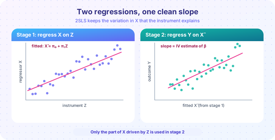
You now know why OLS can be wrong. This lesson shows how to get it right when you have a good instrument. The method is simple enough to state in a sentence: first, use the instrument to predict the endogenous regressor; second, use the prediction instead of the regressor itself. Because the prediction is built only from the instrument, it carries none of the contamination from the error term.
That sentence hides several subtleties: what makes an instrument valid, why the second-stage standard errors printed by a naive two-step procedure are wrong, and what the final number actually estimates. We build everything from the simplest case up.
What you will learn
- The relevance, exogeneity and exclusion conditions for an instrument.
- The simple IV (Wald) estimator
Cov(Z, Y) / Cov(Z, X)and why it works. - How 2SLS handles control variables and several instruments.
- Why second-stage standard errors need correction, and how to interpret the result.
Key terms
First stage: the regression of the endogenous regressor on the instruments and the exogenous controls. Reduced form: the regression of the outcome directly on the instruments and controls. Exclusion restriction: the instrument affects y only through x. Just-identified: as many instruments as endogenous regressors. Overidentified: more instruments than needed. LATE: local average treatment effect, the effect for people whose x the instrument actually moves.
The conditions for a valid instrument
Take the structural equation y = β0 + β1x + u, with Cov(x, u) ≠ 0. A variable z is a valid instrument for x if:
- Relevance:
Cov(z, x) ≠ 0. The instrument must move the regressor. Unlike the other conditions, this one can be tested. - Exogeneity:
Cov(z, u) = 0. The instrument must be unrelated to everything else that influencesy. It must be "as good as randomly assigned" relative to the omitted drivers. - Exclusion:
zdoes not appear in the equation fory. Its only road to the outcome runs throughx.
Conditions 2 and 3 are often discussed together: together they say that z is uncorrelated with the error of the equation we want. They cannot be tested with a single instrument; they are arguments about the real world, supported by institutional knowledge, natural experiments and theory.
The simple IV estimator
Multiply the structural equation by z and take covariances:
Cov(z, y) = β1 Cov(z, x) + Cov(z, u)
With exogeneity, Cov(z, u) = 0, so
β1 = Cov(z, y) / Cov(z, x)
The sample analogue is the IV estimator b1_IV = Σ(zi − z̄)(yi − ȳ) / Σ(zi − z̄)(xi − x̄). In words: the effect of the instrument on the outcome, divided by the effect of the instrument on the regressor. The numerator is the slope of the reduced form and the denominator is the slope of the first stage, so β1 = reduced form / first stage. If the instrument is binary the ratio is the Wald estimator: the difference in mean outcomes between the two instrument groups, divided by the difference in mean x.
Intuition: suppose nearness to a college raises schooling by 0.5 years and raises log wages by 0.04. Then each extra year of schooling, as induced by nearness, raises log wages by 0.04 / 0.5 = 0.08, an eight percent return.
Relevance matters because the denominator is Cov(z, x): if it is close to zero, the ratio explodes and tiny violations of exogeneity produce enormous bias. This is the weak instrument problem of the next lesson.
Two stages
With controls and several instruments we need the general recipe. Let x be the endogenous regressor, w a vector of exogenous controls (including the constant), and z1, ..., zm the excluded instruments.
Stage 1. Regress x on all the exogenous variables w and all the instruments z:
x = π0 + π'w + θ1z1 + ... + θm zm + v, and keep the fitted values x̂.
Stage 2. Regress y on x̂ and the controls w:
y = β0 + β1 x̂ + γ'w + error.
The coefficient on x̂ is the 2SLS estimate. In matrix notation, with X = [x, w] and Z = [z, w], P_Z = Z(Z'Z)⁻¹Z' is the projection onto the instrument space and
b_2SLS = (X' P_Z X)⁻¹ X' P_Z y
Two practical rules follow. Every exogenous control in the structural equation must also be in the first stage. Dropping one from stage 1 makes the fitted x̂ correlated with the omitted control and breaks the logic. And you must not put a nonlinear function of a fitted value into the second stage (the "forbidden regression"): for a squared endogenous term, instrument for x² separately, using z² or interactions.
The standard error trap
The second-stage OLS is a computational device. Its residuals are y − b1 x̂ − ..., built from the fitted x̂, whereas the structural error involves the actual x: û = y − b1 x − γ'w. The variance estimate must use the latter. Statistical packages that run 2SLS in one command compute the correct standard errors; if you do the two steps by hand, you must recompute the residuals and the variance yourself. The correct formula is
V̂ = σ̂² (X' P_Z X)⁻¹, where σ̂² = Σ û² / (n − k).
Adding a heteroskedasticity-robust version (the same sandwich logic as chapter 5) is standard.
The two-step trap is not a theoretical nicety: second-stage standard errors can be badly wrong because x̂ has less variation than x, and the residuals computed from x̂ are not the structural residuals.
Doing it by hand
The following simulation has a hidden confounder (ability), a control (experience), and an instrument (nearness to a college). The code performs both stages and compares the naive second-stage standard error with the correct one.
Press Run (or Ctrl + Enter) to see the result here.
Program input · what you'd type while the program runs
Type the answers before you press Run, one per line. Each time the program reads a line (with input()), it gets the next line from this box.
The 2SLS slope should land near 0.10, while OLS is pulled upward by the ability term. The two standard errors differ, which is exactly why you should rely on proper IV routines.
Seeing the two stages
Press Run (or Ctrl + Enter) to see the result here.
Program input · what you'd type while the program runs
Type the answers before you press Run, one per line. Each time the program reads a line (with input()), it gets the next line from this box.
Notice the horizontal spread: the fitted values x̂ are packed into a narrower range than the actual x. That narrowness is the reason IV is less precise than OLS.
What does the estimate mean?
If everyone responded to x in the same way, the 2SLS slope is simply that common effect. In reality, effects differ across people. Imbens and Angrist showed that with heterogeneous effects, a binary instrument and a monotonicity assumption (nobody is pushed away from treatment by the instrument), the IV estimate is the local average treatment effect (LATE): the average effect for the compliers, those whose x actually changes because of the instrument. Different instruments can therefore give different, equally valid answers: they speak about different groups. This is not a flaw; it is a reminder to state whose effect you identified.
Common misconceptions
"I can run two OLS regressions by hand and read the standard error from the second." The point estimate is right, but the printed standard error is wrong because the residuals use the fitted regressor.
"More instruments are always better." Weak or invalid extra instruments add bias; the extra ones also have to be defended.
"The IV estimate is the effect for everybody." With heterogeneous effects it is the effect for the compliers.
Check your understanding
Quick check · 5 questions
of 5 answered You scored / 5 · perfect!
-
1. Which pair of conditions can be partly tested with data?
Relevance is testable in the first stage. With one instrument, exogeneity and exclusion rest on argument. -
2. The reduced-form slope is 0.04 and the first-stage slope is 0.5. What is the simple IV estimate?
IV = reduced form / first stage = 0.04 / 0.5 = 0.08. -
3. Which statement about controls in 2SLS is correct?
Leaving a control out of stage 1 makes the fitted regressor correlated with that omitted control and breaks the logic. -
4. Why are the standard errors from a hand-run second stage wrong?
The structural error involves the actual x, so the variance must use residuals y - X b. -
5. With heterogeneous effects, the IV estimate with a binary instrument is the effect for...
Under monotonicity, IV identifies the local average treatment effect for those moved by the instrument.
Summary
- A valid instrument is relevant, exogenous and excluded; relevance is testable, the rest is argued.
- The simple IV estimator is the reduced-form slope divided by the first-stage slope.
- 2SLS regresses
xon all instruments and controls, thenyon the fittedxand the controls; use proper standard errors. - With heterogeneous effects, IV estimates the effect for compliers (LATE).
Next: Testing instruments
Track your progress
Create a free account to tick off lessons and pick up where you left off on any device.
of Econometrics lessons completed