


















Lesson 29 of 49 · Instrumental Variables and Endogeneity
Chapter 6 overview: instruments and endogeneity
A map of chapter 6: why endogenous regressors bias OLS, how an instrument isolates clean variation, and how to test whether an instrument is any good.
Chapter 5 dealt with problems of variance: your coefficients were fine, only the error bars were wrong. Chapter 6 is about a much more serious problem, bias. A regressor is endogenous when it is correlated with the error term. Then OLS does not merely give noisy answers; it converges to the wrong number, and collecting more data only makes you more certain of the wrong value.
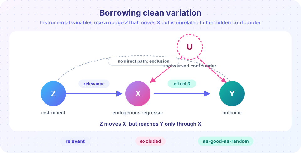
Endogeneity is the central obstacle to learning about cause and effect from non-experimental data. Does an extra year of schooling raise wages, or do able people simply obtain more schooling and also earn more? Does a higher price reduce demand, or do prices rise when demand rises? Does police presence reduce crime, or do cities with more crime hire more police? In each case the regressor of interest is tangled up with something hidden in the error. The tool of this chapter, instrumental variables (IV), untangles it by borrowing variation from a third variable that nudges the regressor without touching the outcome by any other route.
What you will learn
- What endogeneity is, and why OLS is biased and inconsistent under it.
- The three standard sources of endogeneity: omitted variables, measurement error and simultaneity.
- The logic of an instrument, and the two conditions it must meet.
- How two-stage least squares computes the estimate, and how to test an instrument.
Key terms
Endogenous regressor: a regressor correlated with the error term. Instrument Z: a variable that is correlated with the endogenous regressor (relevance) and uncorrelated with the error (exogeneity), affecting the outcome only through the regressor (exclusion). 2SLS: two-stage least squares. Identification: having enough valid instruments to pin the coefficient down. Confounder: a variable that influences both the regressor and the outcome.
The chapter in five slides
The problem
Three roads
The idea
The method
The checks
The core idea in one paragraph
Imagine regressing wages on years of schooling. People with high unobserved ability tend to get more schooling and earn more at any schooling level, so ability sits in the error term and is positively correlated with schooling. OLS attributes part of the ability premium to schooling. Now suppose some people get more schooling for a reason unrelated to ability, for example because a college happens to be built near their home. The extra schooling caused by living near a college is "clean": it is not driven by ability. If we compare wages across people whose schooling differs only because of distance, any wage difference reflects the effect of schooling, not of ability. IV makes this comparison precise: it scales the effect of the instrument on wages by the effect of the instrument on schooling.
A first look at the bias
In the simulation below, the true return to schooling is exactly 0.10 (ten percent per year), and unobserved ability pushes both schooling and wages. OLS misses the truth. A simple IV estimate, the ratio Cov(Z, Y) / Cov(Z, X), comes much closer. These are invented data used only to show the mechanism.
Press Run (or Ctrl + Enter) to see the result here.
Program input · what you'd type while the program runs
Type the answers before you press Run, one per line. Each time the program reads a line (with input()), it gets the next line from this box.
The OLS histogram sits to the right of the dashed line: this is the ability bias. The IV histogram is centred on the truth but is wider, which previews an important theme: IV buys a lack of bias with a loss of precision.
What each lesson covers
- Three roads to endogeneity: omitted variables, measurement error and simultaneity, with the direction of the bias in each.
- Two-stage least squares: the instrument conditions, the Wald ratio, the two stages, and what the estimate means.
- Testing instruments: weak instruments and the first-stage F, overidentification tests and the Hausman test.
- Chapter review: a one-page summary and a ten-question quiz.
Common misconceptions
"A bigger sample cures endogeneity." It does not. A larger sample makes the biased OLS estimate more precise; consistency fails.
"Any variable correlated with X is a good instrument." Correlation with X is only half of what is needed. The instrument must also be unrelated to the error and have no direct effect on Y.
Check your understanding
Quick check · 4 questions
of 4 answered You scored / 4 · perfect!
-
1. A regressor is endogenous when...
Endogeneity means Cov(X, u) is not zero, which makes OLS biased and inconsistent. -
2. In the schooling example, why is OLS biased upward?
Ability is in the error and positively correlated with schooling, so part of its effect is credited to schooling. -
3. Which pair of conditions must a valid instrument satisfy?
Relevance (Cov(Z, X) not zero) and exogeneity (Cov(Z, u) = 0), plus exclusion from the outcome equation. -
4. What is the main price of using IV rather than OLS?
IV removes the bias but uses only part of the variation in X, so standard errors are larger.
Summary
- Endogeneity means the regressor is correlated with the error, so OLS is biased and inconsistent.
- Typical sources are omitted variables, measurement error and simultaneity.
- An instrument is relevant (moves X) and excluded (no other path to Y).
- IV removes bias at the price of precision; instrument strength and validity must be examined.
Track your progress
Create a free account to tick off lessons and pick up where you left off on any device.
of Econometrics lessons completed