


















Lesson 11 of 49 · Simple and Multiple Regression
Chapter 3 overview: simple and multiple regression
Preview chapter 3: fitting a line by least squares, measuring fit with R-squared, controlling for other variables and using logs, dummies and quadratics, with an interactive line fitter.
Chapter 2 told you what a regression is after: the average of the outcome at each value of the explanatory variable. Chapter 3 shows how to get a good estimate of that from a sample. The method is ordinary least squares, or OLS. It is the most widely used estimator in all of applied economics, and a good part of its appeal is that the central idea fits in one sentence: choose the line that makes the total squared prediction mistake as small as possible.
By the end of the chapter you will be able to fit lines by hand and by computer, read the coefficients correctly, judge how well the line fits, add more explanatory variables, and bend the line with logarithms, squares and dummy variables.
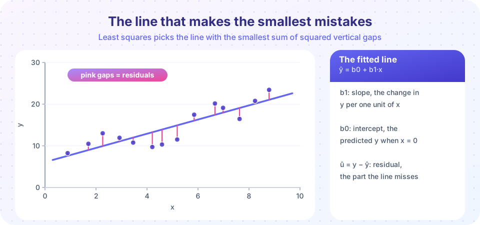
What you will learn
- What each lesson of the chapter covers and how they fit together.
- The vocabulary you will use throughout: fitted value, residual, slope, intercept.
- How to play with a line and see the sum of squared residuals respond.
Key terms
Ordinary least squares (OLS): the method that chooses coefficients to minimize the sum of squared residuals.
Fitted value: the value the line predicts, written ŷ ("y-hat").
Residual: the vertical gap between an observation and the line, û = y − ŷ.
R-squared: the share of the variation in y that the fitted line explains.
The chapter at a glance
One regressor
How good is the fit?
More variables, more shapes
What each lesson covers
- Simple linear regression and OLS derives the slope and intercept formulas, works a five-point example by hand and shows what the residuals must satisfy.
- Goodness of fit and R-squared splits the variation in
yinto explained and unexplained parts and explains what R-squared can and cannot tell you. - Multiple regression adds more variables, explains "holding other things constant", and shows the partialling-out idea behind each coefficient.
- Functional forms, logs and dummies shows how to model percentage effects, curves and group differences with the same machinery.
- Chapter 3 review recaps the chapter and checks it with ten questions.
Before the details: play with a line
The cloud of points below is invented. Drag the intercept and slope sliders to try your own line, and watch the sum of squared residuals, the total of the squared vertical gaps. Then press the button to jump to the OLS line and compare. You will find that no choice of sliders beats OLS, which is its definition.
The next example computes the same OLS line with the formula you will derive in Lesson 1 and checks it against numpy's built-in fit.
Press Run (or Ctrl + Enter) to see the result here.
Program input · what you'd type while the program runs
Type the answers before you press Run, one per line. Each time the program reads a line (with input()), it gets the next line from this box.
Common misconceptions
"OLS finds the true line." OLS finds the line that best fits this sample. Whether it is close to the true line is a question of bias and variance, covered in Chapter 4.
"Least squares is the only reasonable way to fit a line." Other criteria exist, for instance minimizing absolute errors. OLS is popular because it has a simple formula, nice statistical properties and a clear link to averages.
Check your understanding
Quick check · 4 questions
of 4 answered You scored / 4 · perfect!
-
1. What does ordinary least squares minimize?
OLS chooses the intercept and slope that make the total of squared vertical gaps as small as possible. -
2. A residual is
û = y − ŷ is the part of the observation that the line does not capture. -
3. Which lesson explains what R-squared can and cannot tell you?
Lesson 2 of this chapter covers R-squared and its limits. -
4. In the interactive example, can any pair of slider values give a smaller sum of squares than the OLS line?
OLS is defined as the minimizer, so no line has a smaller sum of squares on the same data.
Summary
- OLS fits the line that minimizes the sum of squared residuals.
- A fitted value is the line's prediction; a residual is the observed value minus the fitted value.
- The chapter covers one regressor, fit, multiple regressors and flexible functional forms.
- The sample line is an estimate; its closeness to the truth is the subject of Chapter 4.
Track your progress
Create a free account to tick off lessons and pick up where you left off on any device.
of Econometrics lessons completed