


















Lesson 4 of 49 · Getting Started
A first look at data in Python
Learn the exploratory routine every econometric analysis starts with: inspect, summarize, plot and check correlations, using runnable numpy, pandas and matplotlib code.
Experienced analysts spend more time looking at data than modeling it. A plot can reveal in ten seconds what a regression table hides: a single wild outlier, two clusters you thought were one, a relationship that bends, a column in which missing values were coded as -999. A model fed with data you have not examined is a model you cannot trust.
This lesson gives you a short exploration routine you can use on any data set, plus the few Python tools it needs. You will use numpy for arrays, pandas for tables and matplotlib for pictures, and you can run everything in the browser.
What you will learn
- A five-step routine: inspect, summarize, plot, check relationships, note concerns.
- How to compute and interpret mean, standard deviation, quantiles and correlation.
- How to spot outliers, skewness and missing values.
- Why summary numbers can mislead, and why you must always plot.
Key terms
Mean: the sum of values divided by their count; the balance point of the data.
Standard deviation: a typical distance of values from the mean.
Quantile (percentile): the value below which a given share of observations fall; the 50th percentile is the median.
Correlation: a number between -1 and 1 measuring the strength and direction of a linear relationship.
Outlier: an observation far from the rest, which may be an error or a genuine extreme case.
The routine
Step 1: Inspect. How many rows and columns? What does each column mean, and in what units? What type is each (numbers, text, dates)? Print the first few rows and the column types. In pandas, df.head(), df.shape, df.dtypes and df.info() do this.
Step 2: Check missing and impossible values. Count missing entries in each column with df.isna().sum(). Look for impossible values: negative ages, schooling of 80 years, a wage of zero for a full-time worker. Data sets use special codes for "missing" (such as -9, 999 or "NA"), and averaging those codes in silently ruins results.
Step 3: Summarize. Compute the mean, standard deviation, minimum, quartiles and maximum of every numeric variable. df.describe() produces them all at once. Compare the mean with the median: if the mean is far above the median, the distribution is right-skewed, typical of incomes and prices, because a few very large values pull the mean up.
Step 4: Plot. Draw a histogram of each important variable and a scatterplot of the outcome against the main explanatory variable. Plot first, calculate afterwards.
Step 5: Relationships. Compute correlations and group means (average wage by schooling level). These preview what the regression will show.
Summary statistics, by hand
For n observations x1, ..., xn:
mean:                 x̄ = (x1 + x2 + ... + xn) / n
sample variance:      s² = Σ (xi − x̄)² / (n − 1)
standard deviation:   s  = √s²
correlation:          r  = Σ (xi − x̄)(yi − ȳ) / ((n − 1) · sx · sy)
Why divide by n − 1 and not n in the variance? Because the deviations are measured from the sample mean, which is itself fitted to the same data and sits closer to the observations than the true mean would. Dividing by n − 1 corrects the resulting underestimate of the spread. Chapter 2 shows exactly why.
Worked example
Take five wages in dollars per hour: 12, 15, 18, 20, 35.
- The mean is
(12 + 15 + 18 + 20 + 35) / 5 = 100 / 5 = 20. - The deviations from 20 are
-8, -5, -2, 0, 15; their squares are64, 25, 4, 0, 225, which sum to318. - The sample variance is
318 / 4 = 79.5, so the standard deviation is about8.92. - The median (middle value) is
18, lower than the mean, because of the single high wage of35.
Notice how one value (35) moves the mean and the standard deviation a great deal but leaves the median at 18. Statisticians say the median is robust to outliers and the mean is not. Reporting both tells the reader about skewness.
Correlation, and what it misses
The correlation r has a clear reading: r = 1 means a perfect rising straight line, r = -1 a perfect falling one, and r = 0 no linear relationship. Values like 0.3 are a weak positive association, 0.7 a strong one.
But correlation is only a summary of linear association, and it can mislead. The statistician Francis Anscombe published four small data sets in 1973 that share almost identical means, variances, correlation and fitted line, yet look completely different when plotted: one is a clean line, one a curve, one a line spoiled by a single outlier, one a vertical stack with a single leverage point. Whenever you see a correlation, ask whether you have looked at the scatterplot.
Also remember that correlation is symmetric (the correlation of x with y equals that of y with x), while causation is directional. Ice cream sales and drownings are correlated across months because both rise in summer; neither causes the other. The hidden third factor, temperature, is a confounder.
A tidy way to explore with pandas
Two commands do most of the work. describe() gives the summary table, and groupby() splits the data by a category and summarizes each piece. Suppose you have wages and schooling for many workers: df.groupby("educ")["wage"].mean() returns the average wage at each schooling level, which is the first picture of what the regression will later fit with a straight line. In Chapter 2 you will meet this exact object under the name conditional expectation.
For missing values you have three honest options: drop rows with missing data (fine when few are missing and the reason is unrelated to the outcome), fill them in with a sensible value (and say so), or model the missingness. Never fill silently.
Common misconceptions
"A correlation of 0 means no relationship." It means no linear relationship. A perfect U-shaped relationship can have a correlation of exactly zero.
"Outliers should always be deleted." An outlier may be a typing error, but it may also be the most informative point you have, such as a country in crisis. Investigate, report, and show results with and without it.
"If the mean and the standard deviation match across two data sets, the data sets are alike." Anscombe's data sets show otherwise. Plot them.
Try it
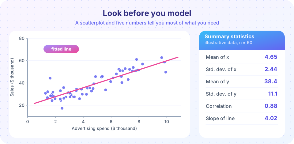
The first example runs the full routine on an invented data set of 60 shops, with sales that rise with advertising. It prints the summary table, the correlation and the fitted slope.
Press Run (or Ctrl + Enter) to see the result here.
Program input · what you'd type while the program runs
Type the answers before you press Run, one per line. Each time the program reads a line (with input()), it gets the next line from this box.
The second example plots a histogram and a scatterplot side by side. In the histogram, check whether the shape is roughly symmetric; in the scatterplot, check whether a straight line is a fair description.
Press Run (or Ctrl + Enter) to see the result here.
Program input · what you'd type while the program runs
Type the answers before you press Run, one per line. Each time the program reads a line (with input()), it gets the next line from this box.
The third example is Anscombe's lesson in miniature. We build two different data sets with the same correlation and show why only a plot reveals the difference. Here one set is a clean line with noise and the other is the same line spoiled by one extreme point.
Press Run (or Ctrl + Enter) to see the result here.
Program input · what you'd type while the program runs
Type the answers before you press Run, one per line. Each time the program reads a line (with input()), it gets the next line from this box.
Check your understanding
Quick check · 5 questions
of 5 answered You scored / 5 · perfect!
-
1. The mean of a wage sample is much larger than its median. This suggests that the distribution is
A few very high wages raise the mean but barely move the median, which is typical of income data. -
2. Why does the sample variance divide by n − 1?
The sample mean is fitted to the same data, so squared deviations from it understate the true spread. -
3. A correlation of 0 between x and y means
Correlation measures linear association only; a U-shaped relationship can have zero correlation. -
4. What should you do first with a new data set?
Looking before modeling catches errors, outliers and shapes that would mislead a regression. -
5. In the worked example (12, 15, 18, 20, 35) the median is 18 because
With five values the median is the third one in sorted order.
Summary
- Start every analysis by inspecting, checking missing or impossible values, summarizing, plotting and checking relationships.
- The mean and standard deviation are sensitive to outliers; the median and quartiles are robust.
- Correlation summarizes only linear association and can be dominated by one point.
- pandas
describe()andgroupby()give the main summaries; matplotlib draws histograms and scatterplots. - Never trust a number you have not seen as a picture.
Next: Chapter 1 review
Track your progress
Create a free account to tick off lessons and pick up where you left off on any device.
of Econometrics lessons completed