


















Lesson 40 of 49 · Computational Aerodynamics
Turbulence modelling, wall spacing and validation
Understand Reynolds averaging, RANS, LES and DNS, how to choose wall spacing with y+, and how grid convergence, verification and validation build trust in CFD.
At the Reynolds numbers of real flight, air does not move in smooth layers. It swirls in a hierarchy of eddies from the size of the wing down to fractions of a millimeter. Resolving all of them with a mesh is impossible for a complete aircraft, so almost every practical CFD result rests on a turbulence model: a set of equations that stands in for the part of the flow the mesh cannot see. This lesson explains the main options, how to design the mesh next to the wall, and how to decide whether to believe an answer.
What you will learn
- How Reynolds averaging creates the closure problem and what RANS models supply.
- The differences between RANS, LES, DES and DNS.
- How to estimate the first-cell height for a target
y⁺. - How grid convergence studies, verification and validation make a result credible.
Key terms
Reynolds stress: extra momentum transport −ρ u'ᵢ u'ⱼ caused by turbulent fluctuations after averaging.
Eddy viscosity (νₜ): a modelled viscosity that mimics the mixing effect of turbulence.
y⁺: dimensionless wall distance y u_τ / ν, with friction velocity u_τ = √(τ_w/ρ).
GCI: grid convergence index, a standard estimate of discretization uncertainty.
Reynolds averaging and the closure problem
Split each velocity into a mean and a fluctuation, u = ū + u', and average the Navier-Stokes equations. The result is the Reynolds-averaged Navier-Stokes (RANS) equations. They look like the original equations for the mean flow, but with one new term, the Reynolds stress, containing unknown correlations of the fluctuations. Now there are more unknowns than equations: the closure problem. A turbulence model supplies the missing relations.
The simplest idea is Boussinesq's eddy viscosity: assume turbulent mixing acts like an extra viscosity, −u'v' = νₜ ∂ū/∂y, and model νₜ with extra transport equations. Common choices:
- Spalart-Allmaras: one equation for a viscosity-like variable; designed for aerodynamics, robust and cheap; widely used for wings and wakes.
- k-ε: equations for turbulent kinetic energy
kand its dissipation rateε; good in free flows, but poor near walls and in adverse pressure gradients without extra wall treatments. - k-ω SST (Menter): blends k-ω near the wall with k-ε far away; the usual choice for flows with pressure gradients and mild separation.
All of these assume the turbulence is near equilibrium. They struggle in strongly separated flow, massive unsteadiness and transition from laminar to turbulent flow (which needs a separate transition model).
Resolving more: LES, DES, DNS
- Large-eddy simulation (LES) resolves the big, energy-carrying eddies in space and time and models only the small ones. It needs a fine, three-dimensional, unsteady mesh and is much costlier than RANS, especially near walls.
- Detached-eddy simulation (DES) and its variants use RANS inside attached boundary layers and LES in separated regions. It is a practical compromise for massively separated flows such as landing gear or high-lift wings.
- Direct numerical simulation (DNS) resolves every scale down to the Kolmogorov scale
η = (ν³/ε)^(1/4). The number of cells grows steeply with Reynolds number, so DNS is limited to simple flows at modestReand serves as "numerical experiments" to build and test models.
Wall spacing and y⁺
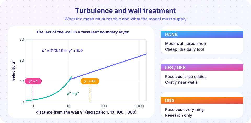
Near the wall the flow structure matters. In wall units the mean velocity is linear in the viscous sublayer (y⁺ < 5), logarithmic in the log layer (y⁺ from about 30 to several hundred), and smoothly joined by a buffer layer in between:
u⁺ = y⁺                                  (y⁺ < 5)
u⁺ = (1/κ) ln y⁺ + B,  κ ≈ 0.41, B ≈ 5.0   (log layer)
There are two standard strategies. Wall-resolved meshes put the first cell center at y⁺ ≈ 1 (or below), so the model integrates through the sublayer: more accurate for separation and heat transfer, but expensive. Wall functions put the first cell in the log layer (y⁺ about 30 to 100) and use the log law as a boundary condition: cheaper, less accurate when the flow separates.
To find the first-cell height: estimate the wall shear from a flat-plate skin-friction correlation (here C_f ≈ 0.026 Re_x^(−1/7)), then τ_w = ½ ρ V² C_f, u_τ = √(τ_w/ρ) and y = y⁺ ν / u_τ. A worked example: a wing of chord 1 m at V = 70 m/s at sea level (ν = 1.46 × 10⁻⁵ m²/s) has Re ≈ 4.8 × 10⁶, C_f ≈ 0.0029, τ_w ≈ 8.7 Pa, u_τ ≈ 2.7 m/s, so y⁺ = 1 corresponds to about 5.5 µm, about five millionths of a meter. That is why wall-resolved boundary-layer meshes have so many thin layers.
Verification, validation and credibility
Two questions must be asked of every simulation, and they are different:
- Verification: are we solving the equations correctly? Checks: does the code reproduce known exact solutions, and does the answer stop changing as the mesh is refined? Mesh refinement studies use at least three grids with a constant refinement ratio
r. With resultsf₁(finest),f₂,f₃the observed order isp = ln((f₃ − f₂)/(f₂ − f₁)) / ln r. Richardson extrapolation estimates the grid-independent valuef_ext = f₁ + (f₁ − f₂)/(rᵖ − 1), and the grid convergence index,GCI = F_s |ε| / (rᵖ − 1)withε = (f₂ − f₁)/f₁and safety factorF_s = 1.25for three grids, quotes the uncertainty. - Validation: are we solving the right equations? Compare with experiments, accounting for experimental uncertainty and tunnel effects. Community events such as the AIAA Drag Prediction Workshops and High Lift Prediction Workshops compare many codes on the same cases, and have shown that results can scatter, especially for separation and drag.
A good CFD report states the mesh, the models, convergence monitors (residuals and force histories), the grid study and the comparison with experiment, with honest uncertainty.
Common misconceptions
"Converged residuals mean a correct answer." They mean the iterative solver has finished; the answer can still be wrong because of the mesh or the model.
"A y⁺ of 1 is always required." It is a target for wall-resolved models; wall functions need the opposite range.
"LES always beats RANS." LES is better for unsteady separated flow, but a bad LES mesh can be worse than a good RANS.
Try it
First, a first-cell height calculator for a flat-plate estimate. Change the speed and chord and the target y⁺.
Press Run (or Ctrl + Enter) to see the result here.
Program input · what you'd type while the program runs
Type the answers before you press Run, one per line. Each time the program reads a line (with input()), it gets the next line from this box.
Second, a grid convergence study. The three drag coefficients are made-up illustrative values; replace them with your own to compute the observed order, the extrapolated value and the GCI.
Press Run (or Ctrl + Enter) to see the result here.
Program input · what you'd type while the program runs
Type the answers before you press Run, one per line. Each time the program reads a line (with input()), it gets the next line from this box.
Check your understanding
Quick check · 5 questions
of 5 answered You scored / 5 · perfect!
-
1. Why does Reynolds averaging create a closure problem?
Averaging nonlinear terms creates unknown fluctuation correlations that need a model. -
2. Which model is the usual choice for aerodynamic flows with adverse pressure gradients?
Menter's SST blends k-ω near the wall with k-ε outside and handles mild separation. -
3. A wall-resolved RANS mesh targets a first cell at about
To integrate through the viscous sublayer the first cell must sit around y⁺ = 1. -
4. Verification asks
Validation compares with reality; verification checks the numerics. -
5. Which method resolves all turbulent scales without modelling?
Direct numerical simulation resolves down to the Kolmogorov scale.
Summary
- RANS replaces the effect of turbulence by a model (Spalart-Allmaras, k-ε, k-ω SST); LES, DES and DNS resolve progressively more.
- Choose the first-cell height from the target
y⁺: about 1 for wall-resolved, 30 to 100 for wall functions. - Verify with grid convergence (observed order, Richardson extrapolation, GCI), then validate against experiment.
Next: Chapter 8 review
Track your progress
Create a free account to tick off lessons and pick up where you left off on any device.
of Aerodynamics lessons completed