


















Lesson 39 of 49 · Computational Aerodynamics
Grids and finite differences
Learn how CFD turns derivatives into arithmetic: finite differences, order of accuracy, the CFL stability limit, numerical diffusion, and grid types and quality.
A computer cannot handle a continuous flow field with infinitely many points. It stores values at a finite set of locations, a grid, and replaces derivatives with differences between neighboring values. This step, discretization, is the heart of CFD. It is also where most numerical error comes from, so understanding what a scheme does to the physics, how accurate it is, and when it blows up, is basic CFD literacy.
What you will learn
- How finite differences follow from Taylor series, and what order of accuracy means.
- How the CFL condition limits the time step of an explicit scheme.
- Why first-order schemes smear and second-order schemes oscillate.
- The main kinds of grid and the measures of grid quality.
Key terms
Discretization: replacing a continuous equation with algebraic equations on a grid.
Order of accuracy (p): the error shrinks like Δxᵖ when the grid spacing Δx shrinks.
CFL number: c Δt / Δx; the number of cells a wave crosses in one time step.
Numerical diffusion: artificial smearing introduced by the scheme, not by the physics.
From Taylor series to differences
Expand a smooth function u about a grid point xᵢ:
u(xᵢ + Δx) = u + Δx·u' + (Δx²/2)·u'' + (Δx³/6)·u''' + ...
u(xᵢ − Δx) = u − Δx·u' + (Δx²/2)·u'' − (Δx³/6)·u''' + ...
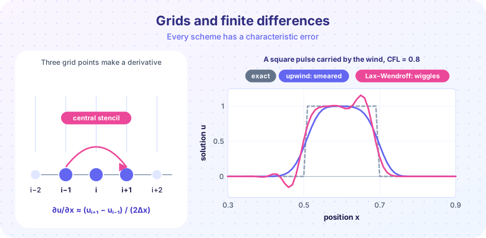
Rearranging the first line gives the forward difference u' ≈ (uᵢ₊₁ − uᵢ)/Δx, with an error term (Δx/2) u'': first order, p = 1. Subtracting the two lines cancels the second-derivative terms and gives the central difference:
u' ≈ (uᵢ₊₁ − uᵢ₋₁) / (2Δx) error ≈ (Δx²/6) u''' second order, p = 2
Halving Δx cuts a first-order error in half, but a second-order error to a quarter. Higher order buys accuracy cheaply on smooth flows but is harder to keep stable and well-behaved near shocks. The set of points used (here i−1, i, i+1) is the stencil.
Three kinds of equation
Flow equations come in three mathematical flavors, and the right numerical approach depends on which one you have:
| Type | Example | Behavior |
|---|---|---|
| Elliptic | Laplace's equation (potential flow), subsonic steady flow | Every point depends on all boundaries; solve everything at once |
| Parabolic | Heat diffusion, boundary layers | Information marches in one direction (time or streamwise) |
| Hyperbolic | Wave and advection equations, supersonic steady flow | Information travels along characteristics (Mach waves) |
The same physical problem can change type: steady flow is elliptic when subsonic and hyperbolic when supersonic. That is why transonic flow with its mixed regions is so awkward to compute.
Marching in time and the CFL limit
Consider the simplest hyperbolic equation, advection: ∂u/∂t + c ∂u/∂x = 0. A pulse simply travels at speed c. An explicit scheme updates each point from known values; the information in one step travels c Δt, and the scheme can only "see" its neighbors Δx away. If the true wave moves further than one cell per step, the scheme cannot capture it and the solution blows up. This is the Courant-Friedrichs-Lewy (CFL) condition:
CFL = c Δt / Δx ≤ 1
Upwind differencing, taking the difference on the side the wind comes from, uᵢⁿ⁺¹ = uᵢⁿ − CFL (uᵢⁿ − uᵢ₋₁ⁿ), is stable for 0 ≤ CFL ≤ 1 and first-order accurate. Its leading error is a diffusion term ½ c Δx (1 − CFL) ∂²u/∂x²: the scheme behaves as if a viscosity were added. That is numerical diffusion, and it is why upwind schemes smear shocks and vortices. The Lax-Wendroff scheme cancels that term and is second order, but its leading error is dispersive (∂³u/∂x³), producing small wiggles near sharp gradients. Modern codes use limiters that blend the two: second order where the flow is smooth, upwind near steep jumps.
A famous theorem, Lax equivalence, ties it together: for a well-posed linear problem, a consistent scheme converges if and only if it is stable.
Finite volumes and conservation
Most production CFD codes use finite volumes: divide the domain into cells and write the conservation laws for the integral over each cell, the flux in minus the flux out. Because whatever leaves one cell enters its neighbor, mass, momentum and energy are conserved exactly, which matters for shocks, where the jump conditions must hold. Finite elements and spectral methods play important roles in structures and research.
Grids and their quality
- Structured grids are indexed by
(i, j, k), like a deformed brick. They are efficient and accurate, but hard to generate around complex shapes. - Unstructured grids (triangles, tetrahedra, polyhedra) fit any geometry and refine easily, at the cost of memory and some accuracy.
- Hybrid grids use thin layers of prisms (a "boundary-layer mesh") next to walls and unstructured cells elsewhere.
- Overset (Chimera) grids overlay separate grids, useful for moving parts such as rotors.
- Adaptive refinement puts cells where the solution changes quickly.
Rules of thumb for quality: avoid high skewness (cells far from regular), keep neighbor size changes smooth (growth ratio of about 1.1 to 1.3 in boundary layers) and keep aspect ratios sensible away from walls. A badly shaped cell can ruin the accuracy of a good scheme.
Common misconceptions
"A finer grid always gives a better answer." Only if the scheme, the model and the geometry are consistent, and roundoff and the time step keep pace. A finer grid with a wrong turbulence model converges to the wrong answer.
"A smooth, beautiful plot means a correct solution." Numerical diffusion produces smooth, plausible but wrong plots.
"Implicit schemes can use any time step so the CFL number is irrelevant." They remain stable at large steps, but accuracy in time still requires resolving the physics.
Try it
First, measure order of accuracy numerically. Compute the derivative of sin x with forward and central differences on successively finer grids, and see how the errors shrink.
Press Run (or Ctrl + Enter) to see the result here.
Program input · what you'd type while the program runs
Type the answers before you press Run, one per line. Each time the program reads a line (with input()), it gets the next line from this box.
Second, advect a square pulse with upwind and Lax-Wendroff and then break the CFL limit.
Press Run (or Ctrl + Enter) to see the result here.
Program input · what you'd type while the program runs
Type the answers before you press Run, one per line. Each time the program reads a line (with input()), it gets the next line from this box.
Check your understanding
Quick check · 5 questions
of 5 answered You scored / 5 · perfect!
-
1. A scheme is second-order accurate. If you halve Δx, the error falls by about a factor of
Error ∝ Δx², so halving Δx gives one quarter. -
2. What does the CFL condition limit?
c Δt / Δx must not exceed 1 for stability of simple explicit schemes. -
3. Upwind differencing smears sharp features because its leading error behaves like
The leading truncation error is a second-derivative term, i.e. diffusion. -
4. Which grid type is best at wrapping around very complex geometry?
Unstructured meshes of tetrahedra or polyhedra can fit any shape. -
5. Supersonic steady flow is described by equations of which type?
Information travels along Mach waves, a hyperbolic character.
Summary
- Finite differences follow from Taylor series; second-order central differences cut error by 4 when
Δxis halved. - Explicit schemes need
CFL ≤ 1; upwind is stable but diffusive, Lax-Wendroff is sharper but dispersive. - Finite volumes conserve mass, momentum and energy; grid type and quality matter as much as the scheme.
Track your progress
Create a free account to tick off lessons and pick up where you left off on any device.
of Aerodynamics lessons completed