


















Lesson 43 of 46 · Projects and Practice
Project: model predator and prey cycles
A guided project: build the Lotka-Volterra predator-prey model, solve it numerically, draw time series and phase portraits, and add a carrying capacity.
Animal populations sometimes rise and fall in regular cycles. In the 1920s, Alfred Lotka and Vito Volterra independently proposed a pair of equations that produce such cycles from a simple idea: predators eat prey, so prey numbers fall, then predators starve and their numbers fall, then prey recover, and the cycle repeats. Records of hare and lynx fur sales in Canada, kept by the Hudson's Bay Company for about a century, show ten-year cycles that are often drawn next to this model, although real hare cycles also depend on food supply and other factors.
In this project you will write the model, solve it numerically, read the graphs and test what changes the cycles. Everything here is a mathematical model and not field data.
What you will learn
- How to write predator-prey equations from biological assumptions
- How to solve differential equations numerically with a Runge-Kutta step or
scipy - How to read a time series and a phase portrait
- Why adding a carrying capacity changes cycles into damped oscillations
Key terms
Lotka-Volterra model: two coupled differential equations for a prey population and a predator population. Equilibrium: a state in which both populations stop changing. Phase portrait: a graph of one variable against the other, with time implicit. Numerical integration: approximating a solution by taking many small time steps. Damped oscillation: a cycle that shrinks over time.
Step 1: write down the assumptions
Let x be the number of prey (hares) and y the number of predators (lynx). We assume
- Without predators, prey grow exponentially at rate
a. - Predators catch prey at a rate proportional to meetings,
x·y, with a catching constantb. - Each prey caught turns into new predators at efficiency
d. - Without prey, predators die off at rate
c.
This gives the equations:
dx/dt = a x - b x y
dy/dt = d x y - c y
Setting both to zero gives the equilibrium: x* = c/d and y* = a/b. At that point predator births exactly balance deaths and prey growth exactly balances predation. A small push away from it sends the system into cycles around the equilibrium.
Step 2: solve and plot
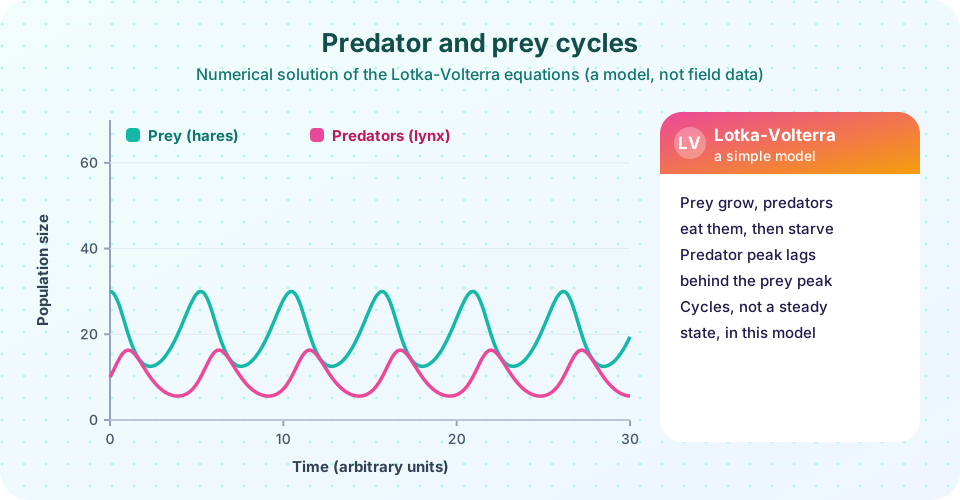
Run the code. It uses the classic textbook values a = 1.0, b = 0.1, c = 1.5, d = 0.075 (the units are arbitrary), then plots the populations over time and as a phase portrait. Try changing the starting numbers. Notice that every starting point gives a closed loop around the equilibrium, but with a different size.
Press Run (or Ctrl + Enter) to see the result here.
Program input · what you'd type while the program runs
Type the answers before you press Run, one per line. Each time the program reads a line (with input()), it gets the next line from this box.
Step 3: read the graph
Three things stand out. The cycles repeat with a steady period. Predators peak after prey, because they need time to turn meals into offspring. And the loop in the phase portrait runs counterclockwise: prey rise first, then predators rise while prey fall, then both fall, then prey recover as predators are scarce.
The model is deliberately simple, and its cycles have an odd property: they never shrink or grow, and each starting point has its own permanent loop. Real populations are not so neutral. That prompts a better model.
Step 4: add a carrying capacity
Prey cannot grow forever, even without predators, because food runs out. Replace the prey growth term a x with the logistic form a x (1 - x/K):
dx/dt = a x (1 - x/K) - b x y
dy/dt = d x y - c y
With a finite K, the cycles tend to damp out and settle at a steady equilibrium, as a result of density dependence. Compare the two models side by side.
Press Run (or Ctrl + Enter) to see the result here.
Program input · what you'd type while the program runs
Type the answers before you press Run, one per line. Each time the program reads a line (with input()), it gets the next line from this box.
Step 5: extensions to try
- Change the starting numbers. Start with only 5 predators. How does the loop size change?
- Change the predator death rate
c. What happens to the equilibrium prey numberc/d? - Find the period. Measure the time between two prey peaks. How does it change when you double
a? - Try other values of K. Is there a K large enough that the cycles look like the classic ones?
- Think like an ecologist. Which assumption is least realistic for hares and lynx? What would you add?
Reading the code and interpreting the results
solve_ivp takes the function that returns the two rates of change, a time span, starting values and a list of times at which to report the answer. The function lv unpacks the current prey and predator numbers and returns dx/dt and dy/dt. The tolerances rtol and atol set how accurate each step must be; very small values give smooth closed loops. The helper find_peaks locates the maxima, so you can measure the period (about five time units here) and the lag between a prey peak and the next predator peak.
The phase portrait is often more revealing than the time series. A closed loop means a repeating cycle. The loop's center is the equilibrium, and the starting point decides how big the loop is. That is why, in this model, a small disturbance such as a hard winter does not die out: the system simply moves to a different loop. In real ecosystems, noise, refuges for prey and limits on predator appetite usually damp or reshape the cycles, which is what the carrying-capacity version shows.
The model also hides a famous puzzle. In 1971 Michael Rosenzweig pointed out that making the prey's environment richer, by raising K in a model like the second one, can destabilize the system and produce larger swings and a greater risk of extinction. He called it the paradox of enrichment. Whether it happens in nature depends on details such as how predators respond when prey are abundant, and field evidence is mixed. It is a good reminder that more food for the prey is not automatically good for the community.
Writing up the project
Describe the biological assumptions first, then the equations, then the parameter values and the solver. Show the time series and phase portrait with labelled axes. State the equilibrium and the period, compare the classic and carrying-capacity versions, and finish with the limits: two species only, constant parameters, no randomness, no space and no age structure. A model is a tool for thinking, so say what it taught you and what it cannot say.
Common misconceptions
"The model predicts the real populations." It shows what a small set of assumptions implies. Real predator-prey systems have many prey, many predators, refuges, disease and weather.
"Predators always follow prey peaks closely." The delay and the size of cycles depend on parameters; some systems show no cycles at all.
"A model that fits a graph proves the mechanism." Different mechanisms can produce similar curves, so a fit is a clue, not proof.
Check your understanding
Quick check · 4 questions
of 4 answered You scored / 4 · perfect!
-
1. In the Lotka-Volterra equations, the term b x y represents...
Encounters between prey and predators, x times y, produce deaths of prey. -
2. What happens to predators when prey become scarce in the model?
Predator births depend on food, so predators fall after prey decline. -
3. Adding a carrying capacity K to the prey tends to...
Density dependence acts as a brake on the swings. -
4. The equilibrium prey number in the classic model is...
Setting dy/dt to zero gives x = c / d.
Summary
- The Lotka-Volterra model couples prey growth and predation to predator births and deaths.
- Numerical integration with
solve_ivpgives time series and phase portraits; the classic model produces closed loops around the equilibrium(c/d, a/b). - Predator peaks lag behind prey peaks.
- Adding a prey carrying capacity damps the cycles; every model leaves out real-world complications.
Next: Glossary
Track your progress
Create a free account to tick off lessons and pick up where you left off on any device.
of Zoology lessons completed