


















Lesson 42 of 46 · Projects and Practice
Project: test the three-quarter rule of metabolic scaling
A guided project: simulate metabolic rates for 40 species, fit the scaling exponent on log-log axes, estimate its uncertainty and compare 3/4 with 2/3.
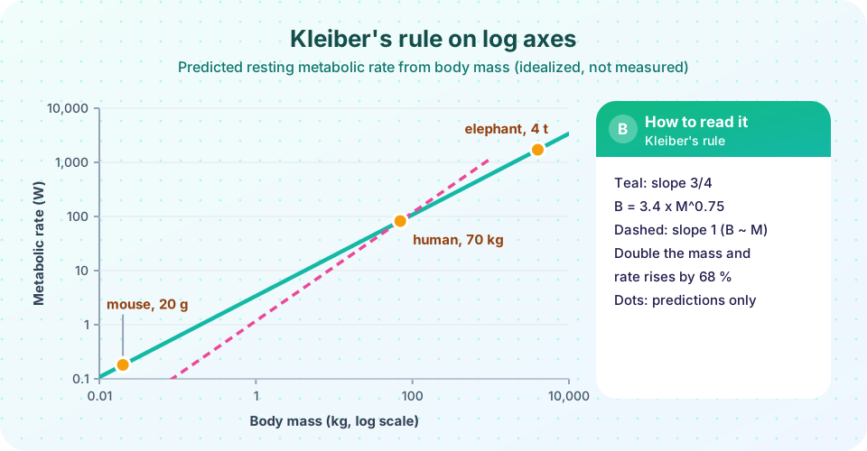
Kleiber's rule says that resting metabolic rate scales with body mass to a power near 0.75. In the physiology chapter you saw what that means for a mouse and an elephant. Now you will do what a researcher would do with a real data table: plot it on log-log axes, fit a straight line, read the exponent from the slope, and ask how sure you can be.
You will not use measured data. The data in this project are simulated from a known rule plus random scatter, which is useful for learning because you know the right answer in advance. With real measurements the same code applies, but the scatter is messier and the conclusions need more care.
What you will learn
- Why power laws look straight on log-log plots and how to read the exponent
- How to fit a line with
numpy.polyfitand describe the scatter - How a bootstrap gives a confidence interval for the exponent
- How to compare competing models such as 3/4 and 2/3
Key terms
Power law: a relationship y = a x^b, where b is the exponent.
Log-log plot: a graph with both axes on logarithmic scales; power laws appear as straight lines.
Regression: fitting a line or curve to data by minimizing errors.
Bootstrap: resampling the data many times to estimate how much a result would vary.
Mass-specific metabolic rate: metabolic rate divided by body mass.
Step 1: why logs?
If B = a M^b, then taking logarithms gives
log B = log a + b × log M
This is the equation of a straight line with intercept log a and slope b. So a power law on a log-log chart is a straight line whose slope is the exponent. A slope of 1 would mean metabolic rate is proportional to mass; a slope of 0.75 means it increases more slowly. Logarithmic axes also let you show animals from shrews to whales in one graph.
Step 2: simulate data
Real metabolic data show scatter because species differ in lifestyle, temperature and diet. We model that as multiplicative noise: the natural log of each rate gets a normally distributed random error with standard deviation 0.25, roughly a quarter on the log scale. The generating rule is B = 3.4 M^0.75 (watts and kilograms). The random generator is seeded so the result is repeatable.
Step 3: fit, bootstrap and compare
Run the next block. Then change true_b or the noise level and see how the estimate and its interval respond.
Press Run (or Ctrl + Enter) to see the result here.
Program input · what you'd type while the program runs
Type the answers before you press Run, one per line. Each time the program reads a line (with input()), it gets the next line from this box.
Step 4: what does the exponent mean?
With an exponent near 0.75, the mass-specific rate (B / M) falls as M^-0.25. Every time mass increases by a factor of 10,000, the per-kilogram metabolic rate drops by a factor of 10,000^0.25 = 10. The mass ratio between a 20 g mouse and a 4,000 kg elephant is 200,000, so the rule predicts that each gram of mouse burns about twenty times more energy than each gram of elephant, even though the mouse's total energy use is tiny. The next block turns the rule into a prediction table with a few familiar animals. The masses are approximate, and the predictions are from the rule, not measurements.
Press Run (or Ctrl + Enter) to see the console output here.
No output.
Step 5: extensions to try
- Change the noise. Set
noise = 0.6. How wide does the bootstrap interval become? Could you still tell 0.75 from 2/3? - Change the sample size. Use
n = 10andn = 200. How does the interval width change? - Add a group effect. Make half of the simulated species ectotherms with a rate ten times lower. What happens to the fitted exponent if you fit all species together and what if you fit the groups separately?
- Explore a different rule. Replace
true_bwith 1. Does the code recover it?
Reading the code and the results
The first block makes a random number generator with a fixed seed, so you and a classmate get the same numbers. It draws 40 log-masses evenly between log10(0.01) and log10(5000), which spreads the species evenly across the graph instead of crowding them among small animals. The rate for each species is the rule value times exp(noise). Because the noise is multiplied, a species can be 25 percent above or below the line, and the scatter looks the same size on a log axis at every body size, as it does in real data.
np.polyfit(x, y, 1) returns the slope and intercept of the least-squares line through the points. Because the points are the logs of the masses and rates, the slope is the exponent and 10 ** intercept is the constant a. In a typical run the estimate lands within a few hundredths of the true value. The bootstrap then draws 2,000 new data sets by sampling species with replacement, refits each, and reports the middle 95 percent of the slopes. If that interval is narrow and sits close to 0.75, the sample strongly supports a slope of about three quarters; if it is wide, the data cannot tell nearby exponents apart.
Notice what the interval does and does not say. It measures the effect of random sampling and scatter on one data set. It cannot tell you whether real animals follow a single power law, whether the true exponent differs among groups, or whether measurement methods were consistent. Researchers who study real metabolic rates argue about all three. Some data sets support 3/4, some 2/3, and some find that the exponent differs between mammals, birds, insects and ectotherms, or between resting and active metabolism.
Writing up the project
A short report has five parts. State the question: does resting metabolic rate scale with mass to about the 0.75 power? Describe the data: how many species, what mass range, what units, and the fact that the data were simulated. Explain the method: log transform, straight-line fit, bootstrap interval. Report the results: slope, constant and interval, with the graph. End with the limits: simulated data, one noise model, no allowance for temperature or phylogeny. Writing the limits is as important as the result.
Common misconceptions
"A straight line on a log-log plot means the relationship is linear." It means a power law; the slope is the exponent, and the original relationship is curved unless the exponent is 1.
"The fit proves the true exponent is exactly 0.75." A fit gives an estimate with uncertainty, and real data from different groups give exponents from about 0.6 to 0.9.
"Simulated data are as good as real data." Simulations teach method and show what the answer should look like, but they say nothing about nature unless they are compared with measurements.
Check your understanding
Quick check · 4 questions
of 4 answered You scored / 4 · perfect!
-
1. On a log-log plot, a power law y = a x^b appears as a straight line with slope...
Taking logs gives log y = log a + b log x, so the slope is the exponent b. -
2. If mass-specific metabolic rate scales as M^-0.25, increasing mass by a factor of 16 reduces it by a factor of...
16 to the 0.25 is 2, so the per-gram rate halves. -
3. What does a wider bootstrap interval indicate?
More variation among resampled fits means less confidence in the slope. -
4. Why simulate data before analyzing real data?
Testing code on data with a known answer reveals mistakes.
Summary
- Taking logs turns the power law
B = a M^binto a straight line whose slope is the exponent. numpy.polyfitestimates the slope; a bootstrap shows how uncertain it is.- An exponent below 1 means mass-specific rate falls with size; a mouse burns far more energy per gram than an elephant.
- Simulated data check your method but are not evidence about nature.
Track your progress
Create a free account to tick off lessons and pick up where you left off on any device.
of Zoology lessons completed