


















Lesson 42 of 46 · Projects and Practice
Project: modeling tumor growth and treatment
Build and compare exponential, logistic and Gompertz tumor growth models in Python, fit one to noisy data, and simulate why resistant cells defeat single-drug therapy.
Chapter 5 told a qualitative story: a tumor starts from one cell, doubles about thirty times before it can be found, and then goes on to invade and spread. In this project you turn that story into numbers. You will build three growth models, fit one of them to simulated measurements, and then run a toy treatment simulation to see why a tumor with a few resistant cells can return after an apparently successful course of treatment.
Everything here is a model: a simplified description built to give insight. Real tumors have a blood supply that varies, immune cells, dying cells, and genetic diversity, so no formula reproduces them exactly. The numbers are invented for teaching, and nothing here is a clinical tool.
What you will learn
- How to write and compare three standard growth models
- How doubling time connects to a growth rate
- How to fit a model to noisy data with scipy
- Why therapy resistance emerges, even when the first response is large
- How to state the limits of a model honestly
Key terms
Doubling time (Td): the time for the population to double.
Carrying capacity (K): the maximum size the environment can support.
Gompertz model: a growth curve in which the growth rate declines steadily as the tumor grows, often used for tumor data.
Log kill: a treatment effect expressed as the fraction of cells killed on a logarithmic scale; "1 log" is a 90 percent kill.
Resistance: survival of cells that the treatment does not harm.
Step 1: three growth laws
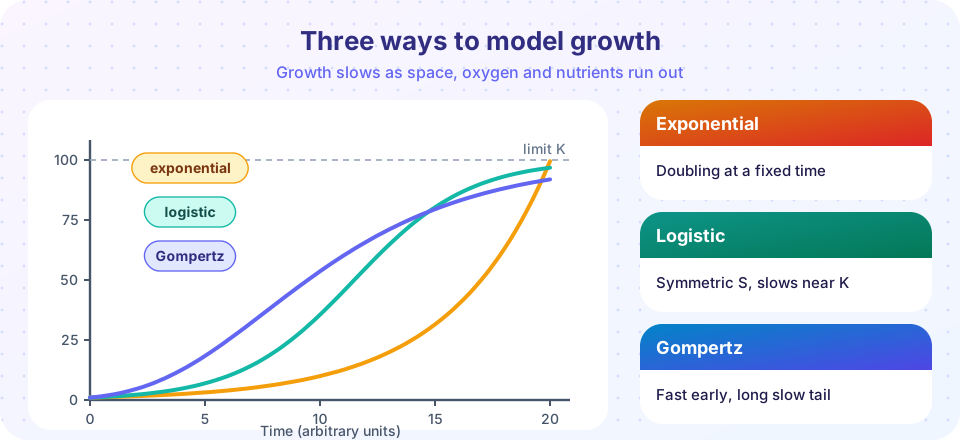
Exponential growth. If every cell divides every Td hours, the number of cells is N(t) = N0 * 2^(t / Td). Equivalently, N(t) = N0 * e^(r t) with a growth rate r = ln(2) / Td. This is exactly what a tumor does in its earliest life, when there is plenty of space and nutrients. It cannot last, because it would soon exceed the size of the body.
Logistic growth. If the growth rate falls linearly as the population approaches a limit K, the curve is an S-shape: N(t) = K / (1 + ((K - N0) / N0) * e^(-r t)). It is symmetric: growth is fastest at half of K.
Gompertz growth. If the growth rate declines exponentially with time, we get N(t) = K * exp( ln(N0 / K) * e^(-a t) ). The curve rises quickly in the early phase and then approaches K slowly, with a long tail. The idea behind it is that a growing tumor has a shrinking fraction of dividing cells (the core gets starved of oxygen). Gompertz curves are widely used to describe tumor growth in animals and in humans, although it is one of several useful models and does not describe every tumor.
Press Run (or Ctrl + Enter) to see the result here.
Program input · what you'd type while the program runs
Type the answers before you press Run, one per line. Each time the program reads a line (with input()), it gets the next line from this box.
Step 2: fit a model to measurements
In practice you have measurements, not formulas. Suppose a mouse tumor is measured every few days. Here we simulate noisy "measurements" from a Gompertz curve with a known answer, so that we can check whether the fit recovers the true parameters. This is a standard way to test a method: use data whose truth you know.
Press Run (or Ctrl + Enter) to see the result here.
Program input · what you'd type while the program runs
Type the answers before you press Run, one per line. Each time the program reads a line (with input()), it gets the next line from this box.
Compare the fitted values with the true ones that the code prints. They land near the truth but not on it, which is what you should expect from noisy data. Look at how the fit behaves. Parameters such as the plateau K are well constrained only when your data reach the plateau. When measurements stop early, many different K values fit almost equally well, and predictions about the future are uncertain. This is a general lesson: a fitted model is good at interpolation, and extrapolation depends on assumptions.
Step 3: a toy treatment simulation
Treatment kills a fraction of cells in every cycle, not a fixed number. Suppose each treatment cycle kills 90 percent of sensitive cells (a "1-log kill"), and that between cycles the surviving cells regrow. A small number of resistant cells may already exist before treatment, because every division carries a small chance of mutation. Resistant cells are not harmed, so they keep growing, and as the sensitive population falls, they take over.
Press Run (or Ctrl + Enter) to see the result here.
Program input · what you'd type while the program runs
Type the answers before you press Run, one per line. Each time the program reads a line (with input()), it gets the next line from this box.
The curve for sensitive cells falls steeply, so the tumor appears to shrink. Meanwhile the resistant cells, hidden below the detection limit, grow every cycle. At some point the lines cross, and the tumor returns, now resistant. Several real strategies are motivated by this picture, without any model being the same as reality: treating early, when fewer resistant cells exist; using several drugs with different mechanisms, so that a cell would need several mutations at once to resist; and combining drugs with surgery or radiotherapy.
Step 4: your own extensions
Try these changes in the code above:
- Change the doubling time. How does the time to reach 10^9 cells change if Td is 30 days rather than 60? (Use the formula
t = Td * log2(N / N0).) - Change the kill fraction. What happens with a 99 percent kill per cycle? What about 50 percent?
- Change the resistant fraction. Set it to 1e-9. How many cycles does it take for resistant cells to dominate?
- Add a second drug that kills the resistant cells but not the sensitive ones, and alternate the drugs.
- Replace the regrowth with a Gompertz recovery. Does the picture change?
Interpreting results honestly
A good modeler writes down what the model leaves out. Our models ignore the immune system, the tumor's blood supply, heterogeneity, drug delivery that varies in space, and the fact that cells die even without treatment. They are valuable because they let you ask "what if?" cheaply, and a wrong model that is clear is easier to improve than a correct model that cannot be understood. They are dangerous when numbers produced by a toy are quoted as facts. When you report a result, state the assumption, the parameter values, and what would make the result fail.
Common misconceptions
- "A model that fits the data is true." Several models can fit the same data, and a good fit does not prove the mechanism.
- "Exponential growth means cancer grows faster than any normal tissue." Many normal tissues renew quickly; cancers differ by failing to stop and by lacking coordination.
- "A large shrinkage means cure." Tumors can shrink while a resistant subpopulation survives.
Check your understanding
Quick check · 4 questions
of 4 answered You scored / 4 · perfect!
-
1. If the doubling time is 60 days, roughly how many days does it take to grow from 10^6 to 10^9 cells?
10^3-fold growth needs log2(1000), about 10 doublings, so about 600 days. -
2. Which curve has a long, slow approach to its limit after a fast early phase?
The Gompertz curve's growth rate declines steadily, giving a long tail. -
3. Why can a treatment that kills 90 percent of cells per cycle still fail?
Pre-existing resistant cells survive and take over as the sensitive cells fall. -
4. A fitted curve is least reliable when
Extrapolation depends on assumptions the data cannot check.
Summary
- Exponential, logistic and Gompertz models capture different aspects of growth; the Gompertz curve has a long slow tail.
- Doubling time and growth rate are linked by
r = ln(2) / Td. - Fitting a model to data works best when the data cover the part of the curve you care about.
- A toy treatment model shows how pre-existing resistant cells explain relapse.
- Models give insight when their assumptions are stated honestly.
Next: Practice problem sets
Track your progress
Create a free account to tick off lessons and pick up where you left off on any device.
of Pathology lessons completed