


















Lesson 40 of 49 · Quality, Automation and Lean
Statistical process control and process capability
Learn how X-bar and R control charts detect process changes, how to compute Cp and Cpk, what the numbers mean in defects per million, and why you should not tamper with a stable process.
Imagine measuring the diameter of every fiftieth shaft that leaves a lathe. The numbers wobble: 25.002, 24.997, 25.004, 24.999. Is that wobble normal, or is something going wrong? If the operator adjusts the machine each time a value looks high, will the shafts get better or worse? Statistical process control (SPC) answers these questions with simple tools built on one insight: a stable process has a predictable amount of variation, and anything beyond that is a signal to investigate.
What you will learn
- The difference between common-cause and special-cause variation.
- How to build X-bar and R control charts and read their signals.
- How to compute Cp and Cpk and convert them to defect rates.
- Why adjusting a stable process makes it worse.
Key terms
Common-cause variation: the natural, ever-present variation of a stable process.
Special-cause variation: variation from a specific, identifiable event (a worn tool, a new batch of material, a loose fixture).
Control limits: limits at three standard deviations of the plotted statistic around its mean; they come from the data, not from the specification.
Specification limits (LSL, USL): limits set by the customer or the designer; they come from requirements, not from the data.
Process capability: how well the spread of the process fits inside the specification limits.
Two kinds of variation
Even a well-run machine produces parts that differ slightly because of tiny, uncontrollable changes: vibration, small differences in the material, temperature. This is common-cause variation. As long as only common causes act, the process is in statistical control: its output follows a stable distribution, and we can predict how it will behave.
When something specific changes, such as a tool starts to wear, a coolant runs low, a new operator sets the fixture differently, the distribution shifts or widens. This is special-cause variation. The purpose of SPC is to detect special causes quickly, so you can find and fix them, and to avoid reacting to common causes.
X-bar and R charts
The classic variables chart pair works on subgroups: take a small sample (often 4 or 5 consecutive parts) at regular intervals, plot the subgroup mean (x̄) on one chart and the subgroup range R (largest minus smallest) on another. The mean chart shows whether the center moves; the range chart shows whether the spread changes.
Limits are computed from a baseline period of about 20 to 25 subgroups when the process is running normally. With x̿ the average of the subgroup means and R̄ the average of the ranges:
X-bar chart:   UCL = x̿ + A2 R̄      LCL = x̿ − A2 R̄
R chart:       UCL = D4 R̄          LCL = D3 R̄
Estimated σ:   σ̂ = R̄ / d2
The constants depend on the subgroup size n:
| n | A2 | D3 | D4 | d2 |
|---|---|---|---|---|
| 4 | 0.729 | 0 | 2.282 | 2.059 |
| 5 | 0.577 | 0 | 2.114 | 2.326 |
| 6 | 0.483 | 0 | 2.004 | 2.534 |
Worked example 1
Twenty-five subgroups of 5 gave x̿ = 25.002 mm and R̄ = 0.024 mm. With n = 5:
UCL = 25.002 + 0.577 × 0.024 = 25.016 mm,LCL = 25.002 − 0.014 = 24.988 mm.- R chart:
UCL = 2.114 × 0.024 = 0.051 mm,LCL = 0. σ̂ = 0.024 / 2.326 = 0.0103 mmfor individual parts.
Note that the control limits (24.988 to 25.016) are for subgroup means, which vary less than individual parts. They are not the tolerance limits of the part.
Signals
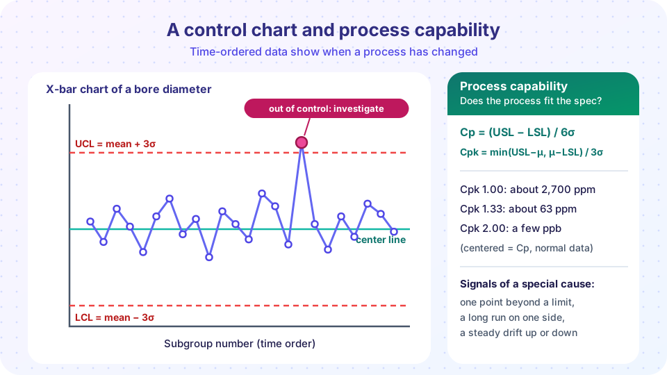
A point is a signal that a special cause is likely when:
- A point falls outside a control limit.
- A long run of points (commonly 7 to 9, depending on the rule set) lies on one side of the center line.
- A trend of six or so points steadily rises or falls.
- Two of three consecutive points are beyond the two-sigma line on the same side.
Different handbooks (Western Electric, Nelson) use slightly different run lengths; whichever set you use, apply it consistently. Each rule is a trade: sensitive rules detect shifts sooner but give more false alarms.
Other charts
| Data | Chart |
|---|---|
| Measurements in subgroups | X-bar and R (or X-bar and S for larger subgroups) |
| Single measurements, one at a time | Individuals and moving range (I-MR) |
| Fraction of defective parts | p chart |
| Number of defects per unit (count) | c or u chart |
Process capability: Cp and Cpk
A process can be in control and still produce bad parts if its spread is wider than the tolerance. Capability indices compare the process spread with the specification:
Cp  = (USL − LSL) / (6σ)
Cpk = min( (USL − μ), (μ − LSL) ) / (3σ)
Cp asks: could the process fit within the limits if it were perfectly centered? Cpk asks the harder question: does it fit given where the mean actually sits? Cpk is never larger than Cp; they are equal when the process is centered.
Worked example 2
Specification 25.00 ± 0.05 mm (so LSL = 24.95, USL = 25.05). The process has μ = 25.012 mm and σ = 0.0103 mm:
Cp = 0.10 / (6 × 0.0103) = 1.62Cpk = min(25.05 − 25.012, 25.012 − 24.95) / (3 × 0.0103) = min(0.038, 0.062) / 0.0309 = 1.23
The process is capable in spread (Cp 1.62) but not well centered, so Cpk is 1.23 and the upper side is the risk. Re-centering the mean at 25.00 would raise Cpk back to 1.62 at no cost.
What numbers mean. For a normal, centered process: Cpk 1.00 gives about 2,700 defective parts per million (ppm) (the two tails beyond ±3σ); Cpk 1.33 about 63 ppm; Cpk 1.67 under 1 ppm; Cpk 2.00 a few parts per billion. Many customers, particularly in the automotive sector, require a minimum Cpk of 1.33 for established characteristics and higher (often 1.67) for new or safety-critical ones. The "6 sigma" target is a Cp of 2, and the quoted 3.4 defects per million comes from assuming a 1.5σ shift in the mean over the long term.
Capability indices only mean something when the process is in control (otherwise σ is not stable), when the data are roughly normal, and when the data come from enough parts (at least 50 to 100 measurements). Long-term versions called Pp and Ppk use the overall standard deviation, including drift between subgroups.
Do not tamper
A tempting reaction is to adjust the machine whenever a part is a little high or a little low. Deming's famous funnel experiment shows why this is harmful: adjusting a stable process in response to common-cause variation increases the variation, in the simplest case by a factor of about 1.4 (√2), because the adjustment adds its own random error to the natural scatter. Adjust only when a control chart gives a signal that something has changed, and try to find why it changed, rather than just compensating.
Common misconceptions
"The control limits are the tolerance limits." Control limits describe what the process does (and for x̄ charts, how subgroup means vary). Specification limits describe what the customer needs. They are independent.
"In control means good." A process can be stable and consistently produce parts outside the tolerance. Control says predictable, capability says acceptable.
"If all the points are inside the limits, nothing is wrong." Runs, trends and patterns can signal trouble well before any point crosses a limit.
Try it
First, simulate a process with a shift partway through. The script builds the limits from the first 20 subgroups and then reports when the chart (or a run rule) first signals.
Press Run (or Ctrl + Enter) to see the result here.
Program input · what you'd type while the program runs
Type the answers before you press Run, one per line. Each time the program reads a line (with input()), it gets the next line from this box.
Second, explore capability. Move the sliders for the mean and the standard deviation, and watch Cp, Cpk and the expected defect rate.
Check your understanding
Quick check · 5 questions
of 5 answered You scored / 5 · perfect!
-
1. A process has USL = 10.30, LSL = 9.70 and σ = 0.05. What is Cp?
Cp = (USL − LSL) / 6σ = 0.60 / 0.30 = 2.00. -
2. For the same process the mean is 10.10. What is Cpk?
Cpk = min(10.30 − 10.10, 10.10 − 9.70) / (3 × 0.05) = min(0.20, 0.40) / 0.15 = 1.33. -
3. What is the best response to a single point that is high but inside the control limits on a stable chart?
A point inside the limits with no pattern is expected variation. Adjusting would add variation (tampering). -
4. With n = 5, R̄ = 0.030 mm and x̿ = 50.000 mm, what is the X-bar chart UCL (A2 = 0.577)?
UCL = x̿ + A2 R̄ = 50.000 + 0.577 × 0.030 = 50.0173 mm. -
5. Which statement about control limits and specification limits is correct?
Control limits are calculated from the process's own variation, specification limits are set by design or the customer.
Summary
- Common-cause variation is natural and predictable; special causes are specific events to find and fix.
- X-bar and R charts with limits
x̿ ± A2 R̄andD4 R̄show shifts in center and spread; rules for runs and trends add sensitivity. Cp = (USL − LSL)/6σcompares spread with tolerance;Cpkalso accounts for centering. Cpk 1.33 is about 63 ppm for a normal process.- Do not tamper: adjusting a stable process increases variation.
Track your progress
Create a free account to tick off lessons and pick up where you left off on any device.
of Manufacturing Processes lessons completed