


















Lesson 7 of 50 · Methods and Cognitive Architecture
Reaction Times and Mental Chronometry
How psychologists time mental processes: Donders and Sternberg, Hick's law, skewed RT distributions, the speed-accuracy trade-off and a decision-process simulation.
If you want to study something invisible, measure how long it takes. Mental chronometry is the use of response times to infer the structure of mental processes. A difference of 30 milliseconds between two conditions, far too small for anyone to notice, can reveal that one task includes an extra step. This is why so many cognitive experiments look like a person pressing keys as quickly as possible while a clock runs.
What you will learn
- The three basic reaction-time tasks and what each measures.
- How Donders's subtractive method and Sternberg's additive-factors logic time mental stages.
- Why reaction times are skewed and how to summarize them.
- What the speed-accuracy trade-off is and why you must always check accuracy.
- Hick's law and a sketch of how decisions can be modeled.
Key terms
Reaction time (RT): the time from a stimulus appearing to the person's response.
Simple RT: one stimulus, one response. Choice RT: several stimuli, each with its own response.
Speed-accuracy trade-off: responding faster tends to produce more errors, and vice versa.
Subtractive method: estimating a stage's duration by subtracting the RT of a task without it from one with it.
Additive-factors method: if two variables add their effects, they affect different stages; if they interact, they affect a shared stage.
Three basic tasks
- Simple reaction time. One signal, one response, such as pressing a key whenever a light turns on. Typical values are around 200 to 250 ms for a light in healthy young adults in the lab, depending on equipment and conditions.
- Go/no-go. Respond to one kind of stimulus, withhold for another. It adds a discrimination step.
- Choice reaction time. Several stimuli, each mapped to a different response (for example, left key for a circle, right key for a square). It adds selection of the response.
Each added requirement adds time. In 1868 the Dutch physician Franciscus Donders used this to propose the subtractive method: the difference between choice RT and simple RT estimates the time to select a response. His reasoning was bold and it was criticized for a good reason: it assumes pure insertion, meaning a stage can be added without changing any other stage. That is often false. Adding a decision requirement can change how people prepare their motor response.
Sternberg and additive factors
In 1966 Saul Sternberg asked people to memorize a short list of digits and then judged whether a test digit was on the list. RT increased in a straight line with the length of the list, by roughly 40 ms per item (the exact value depends on the study), and the line was about equally steep for "yes" and "no" answers. Sternberg proposed that people scan memory serially and exhaustively, checking every item even after a match. This was a striking, testable theory, and later work showed that other models (for example, parallel ones) can sometimes mimic the same line, a reminder of the mimicry problem from Chapter 1.
In 1969 Sternberg proposed the additive-factors method. Suppose you manipulate two variables, such as the clarity of a stimulus and the number of response options.
- If the effects add (making the stimulus unclear slows you by 50 ms whether there are 2 or 4 choices), the variables probably influence different stages.
- If they interact (the effect of clarity is larger with more choices), they probably share a stage.
This replaced the weaker pure-insertion assumption with something that can be checked in the data.
Hick's law
When people choose between more alternatives, RT rises, but by smaller and smaller steps. In 1952 W. E. Hick and, independently, Ray Hyman (1953) described the relation:
RT = a + b × log2(n + 1)
Here n is the number of equally likely alternatives, a is the time for everything unrelated to the choice, and b is the cost of each bit of information. Doubling the choices adds about a constant amount, not double the time. The law helps explain why long menus slow down users, and it is a handy reminder that people handle choices by information, not by item count. It fits many tasks but not all, especially with highly practiced or very natural mappings.
What do RT data look like?
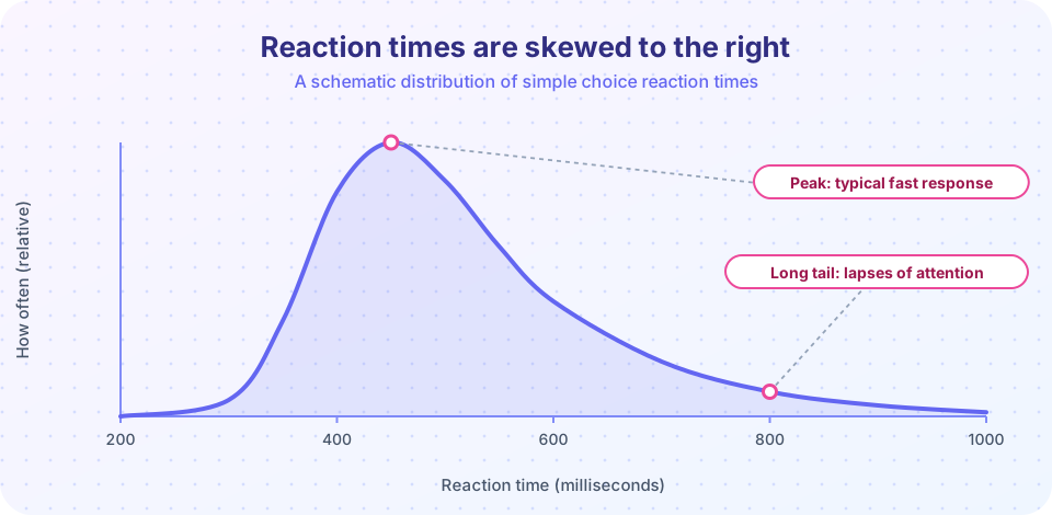
RT distributions are not symmetrical. They have a fast edge (people cannot respond faster than their sensory and motor systems allow), a peak, and a long tail to the right produced by lapses of attention and slow trials. A common description, the ex-Gaussian, is the sum of a normal distribution and an exponential tail.
Because of the tail:
- The mean is pulled up by rare very slow trials. The median is more stable.
- Researchers remove implausible trials: anticipations (for example, under 100-150 ms, too fast to be a real response) and very long outliers. The rules should be decided before looking at the results, so they cannot be tuned to give a desired answer.
- Some analyses use a log transform or fit the whole distribution, because an effect can sit in the leading edge, in the tail, or in both. An effect confined to the tail means occasional slow-downs, not a uniformly slower process.
The speed-accuracy trade-off
People can choose to be fast and sloppy or slow and careful. If condition A shows faster RTs than condition B, but with more errors, you cannot say A is easier: the participants may simply have been less careful. Always examine accuracy together with RT. One way to deal with this is to impose time limits and measure accuracy at several deadlines, forming a speed-accuracy curve. Another is to use models.
The best-known family is the sequential-sampling or drift-diffusion model (Roger Ratcliff and others, from the 1970s). Evidence accumulates noisily toward one of two boundaries. When it hits a boundary, the person responds.
- A higher boundary means more caution: slower but more accurate.
- A higher drift rate means clearer evidence: faster and more accurate.
This simple idea explains the trade-off and the skewed shape of RT distributions together, which is much of why it is so widely used.
A caution about home-made reaction timers. On a normal computer, screen refresh rates, keyboard scanning, browser scheduling and operating-system delays add tens of milliseconds of error that can differ between devices. Careful laboratory work uses calibrated equipment. A web demo can show the idea, but not precise absolute timing.
Common misconceptions
"Faster reaction time means a better brain." A difference between two people, or two days, may reflect caution, motivation, practice or equipment. Within an experiment, differences between conditions are interpretable; single scores are not a measure of intelligence.
"A 10 ms difference is too small to matter." In well-designed experiments with many trials, differences of tens of milliseconds are reliable and informative.
"Use the mean, it is the usual average." With skewed data, the mean can mislead. Check the median and the distribution.
Try it
Press Run (or Ctrl + Enter) to see the result here.
Program input · what you'd type while the program runs
Type the answers before you press Run, one per line. Each time the program reads a line (with input()), it gets the next line from this box.
Press Run (or Ctrl + Enter) to see the result here.
Program input · what you'd type while the program runs
Type the answers before you press Run, one per line. Each time the program reads a line (with input()), it gets the next line from this box.
Press Run (or Ctrl + Enter) to see the console output here.
No output.
Check your understanding
Quick check · 5 questions
of 5 answered You scored / 5 · perfect!
-
1. Donders's subtractive method assumes that
This assumption is called pure insertion, and it is often questionable. -
2. If two experimental variables have additive effects on RT, the additive-factors method suggests they
Additive effects point to separate stages; interactions suggest a shared stage. -
3. Why is the median often preferred to the mean for RT?
A long right tail inflates the mean, while the median is less affected. -
4. In Hick's law, doubling the number of equally likely choices
RT grows with the logarithm of the number of choices, so each doubling adds about the same time. -
5. Condition A has faster RTs than condition B but more errors. The best conclusion is that
A speed-accuracy trade-off could explain the pattern, so accuracy and RT must be interpreted together.
Summary
- Response times reveal the structure of mental processes; small differences can be meaningful.
- Donders's subtraction and Sternberg's additive factors are two logics for timing stages, each with assumptions.
- Hick's law relates choice RT to the logarithm of the number of alternatives.
- RT is right-skewed: use medians, look at distributions, and set exclusion rules in advance.
- Always read accuracy together with RT; drift-diffusion models capture the trade-off.
Track your progress
Create a free account to tick off lessons and pick up where you left off on any device.
of Cognitive Psychology lessons completed