


















Lesson 37 of 50 · Reasoning, Judgment and Decision Making
Probability and Bayes
Learn how evidence should change belief: base rates, Bayes' rule, the screening-test problem, natural frequencies, conservatism, overconfidence and the hot hand, with a calculator.
A medical screening test is positive. How worried should you be? Most people, including many doctors in early surveys, answer by looking at how accurate the test is. But the right answer also depends on something that rarely feels relevant: how common the condition is in the first place. Combining prior knowledge with new evidence is the job of Bayes' rule, and it is the main tool for judging how much to believe something. This lesson shows the rule, the classic way people get it wrong, and a simple trick that helps.
What you will learn
- What a base rate, a likelihood and a posterior probability are.
- How to apply Bayes' rule with probabilities and with natural frequencies.
- Why the screening problem confuses people and how to teach it better.
- Other known patterns: conservatism, overconfidence and the hot hand.
Key terms
Prior probability (base rate): how likely something is before seeing new evidence.
Likelihood: how probable the evidence is if the hypothesis is true.
Posterior probability: the probability of the hypothesis after considering the evidence.
Sensitivity: the chance that a test is positive when the condition is present.
False positive rate: the chance that a test is positive when the condition is absent.
Bayes' rule
Thomas Bayes' rule, published after his death in 1763, says that the probability of a hypothesis H after seeing evidence E is:
P(H | E) = P(E | H) × P(H) / P(E)
where P(E) adds up all the ways to get the evidence: P(E) = P(E | H) × P(H) + P(E | not H) × P(not H). In words: posterior = likelihood × prior, scaled so that the possibilities sum to one. An equivalent form uses odds: posterior odds = prior odds × likelihood ratio. The important message is that the same evidence can lead to very different conclusions when priors differ.
The screening problem
David Eddy (1982) described a problem in the style of mammography screening: about 1 percent of women in a group have a condition; the test is positive for 80 percent of women who have it; and it is also positive for 9.6 percent of women who do not. A woman tests positive. What is the chance that she has the condition?
Compute it. P(positive) = 0.80 × 0.01 + 0.096 × 0.99 = 0.008 + 0.09504 = 0.10304, so P(condition | positive) = 0.008 / 0.10304, about 0.078, or 7.8 percent. In Eddy's informal survey, most physicians gave an answer close to 75 percent, mistaking the test's sensitivity for the chance that a positive result is correct. This is the base-rate neglect of the previous lesson in a high-stakes setting. The test is quite good at detecting the condition, but the condition is rare, so most positives come from the large group of people who do not have it.
Natural frequencies
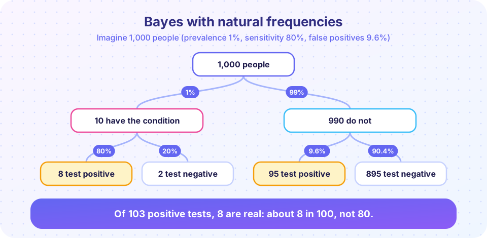
Gerd Gigerenzer and Ulrich Hoffrage (1995) showed that the same problem becomes far easier when restated in natural frequencies, which are counts of people. Imagine 1,000 people. About 10 have the condition, and 8 of them test positive. Of the 990 who do not, about 95 test positive. So among the 103 positives, 8 are real: about 8 in 100. In their studies, the proportion of correct Bayesian answers roughly tripled with natural frequencies compared with probability wording (people were still not perfect). Natural frequencies match the way we have encountered information through experience, and they make the "denominator" visible. Practical lesson: when communicating risk, use counts out of a fixed group (for example, "8 of 103") instead of chains of percentages.
Other patterns in probability judgment
- Conservatism. In some laboratory tasks, people revise their beliefs less than Bayes' rule says they should (Ward Edwards, 1968). Yet in other tasks, such as when evidence is vivid, they revise too much, so there is no single direction of error.
- Overconfidence and calibration. When people say they are 90 percent sure, they are often right far less than 90 percent of the time. Overconfidence is common for hard questions and in experts whose feedback is slow or absent. Weather forecasters, who get daily feedback, are unusually well calibrated.
- Randomness and the hot hand. People expect random sequences to alternate more than they do, so streaks look meaningful. Gilovich, Vallone and Tversky (1985) concluded that basketball shooters have no "hot hand". A later reanalysis (Miller and Sanjurjo, 2018) found that the original method was biased against finding streaks, so a small real effect may exist. The episode illustrates how subtle statistics can be, even for experts.
- Illusory correlation and confirmation. We notice and remember cases that fit an expected pattern more than cases that do not.
Improving probabilistic thinking
Evidence-based aids include natural frequencies, icon arrays (grids of 100 or 1,000 people with the affected people shaded), asking "out of how many?" and thinking of base rates first. Teaching Bayes' rule with frequency formats has lasting benefits in studies of medical students and judges. These skills matter for anyone who reads research, because a significant result in a field where few hypotheses are true can be a false positive more often than the p-value suggests (see chapter 9).
Common misconceptions
"A positive test with 80 percent sensitivity means 80 percent chance of having the condition." The chance depends on the base rate and the false positive rate.
"A 95 percent accurate test is wrong 5 percent of the time, so a positive is 95 percent right." "Accuracy" mixes sensitivity and false positives; the right quantity is the positive predictive value.
"Bayes' rule is only for statisticians." It is a rule for updating beliefs, and it can be used with counts and trees without any formula.
Try it
Press Run (or Ctrl + Enter) to see the result here.
Program input · what you'd type while the program runs
Type the answers before you press Run, one per line. Each time the program reads a line (with input()), it gets the next line from this box.
Check your understanding
Quick check · 5 questions
of 5 answered You scored / 5 · perfect!
-
1. In Bayes' rule, the posterior probability combines
Posterior is proportional to prior times likelihood. -
2. With 1% prevalence, 80% sensitivity and 9.6% false positives, the chance of the condition after a positive test is about
0.008 / (0.008 + 0.09504) is about 0.078. -
3. Natural frequencies help because they
Gigerenzer and Hoffrage found much better Bayesian reasoning with frequency formats. -
4. Overconfidence means that
When people say 90% sure, they are often right less often than that. -
5. The hot hand reanalysis by Miller and Sanjurjo (2018) showed that
A subtle statistical bias had affected the original conclusion.
Summary
- Bayes' rule combines a prior (base rate) with the likelihood of evidence to give a posterior.
- When a condition is rare, most positive tests can be false positives, even for a fairly accurate test.
- Natural frequencies and trees make Bayesian reasoning easier than percentages.
- Other known patterns include conservatism, overconfidence and misjudging randomness, and the evidence on them is nuanced.
Track your progress
Create a free account to tick off lessons and pick up where you left off on any device.
of Cognitive Psychology lessons completed