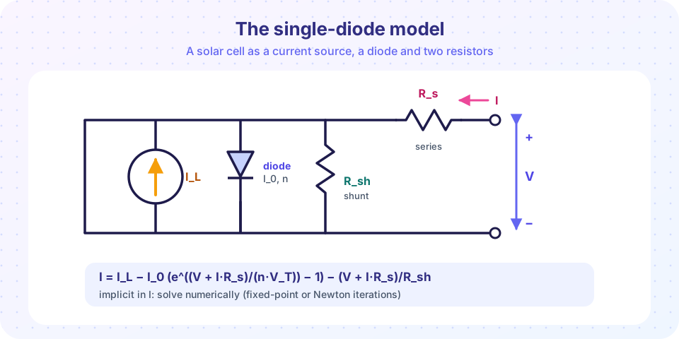
Build a single-diode solar cell model with series and shunt resistance, extract efficiency and fill factor, fit it to noisy data and study temperature and irradiance effects.
Solar-cell engineers, module manufacturers and energy modelers all use the same simple circuit to describe a cell: a current source, a diode and two resistors. In this project you will build that single-diode model, extract the headline numbers from it, fit its four parameters to noisy "measured" data (the way a lab does), and then explore how temperature and light intensity change the picture.
Caption: The photocurrent I_L flows in parallel with the diode and the shunt resistance; the series resistance sits between the junction and the terminals.
Because J appears on both sides, we cannot solve it algebraically without special functions. A root finder solves it point by point: for each voltage V, find the J that makes the left side equal the right side. We work per unit area (A/cm², Ω·cm²), so the cell size drops out.
A lab measures a cell and wants the four hidden parameters J_L, J_0, R_s and R_sh. The standard approach is nonlinear least squares: adjust the parameters until the model matches the data. Because J_0 spans many orders of magnitude, fit its logarithm. Here we generate "measurements" from known parameters with 0.3% noise and see whether the fit recovers them.
Press Run (or Ctrl + Enter) to see the result here.
Program input · what you'd type while the program runs
Type the answers before you press Run, one per line. Each time the program reads a line (with input()), it gets the next line from this box.
Two cautions that every experimentalist learns. First, the fit is only as good as the data range: R_sh is set by the nearly flat low-voltage region and R_s by the steep region near V_oc, so data must cover both. Second, the ideality factor n and J_0 are strongly correlated; fixing n (as here) or fitting data at several temperatures avoids a family of equally good but physically different answers.
Cells in the field are not at 25 °C and 1 sun. Temperature raises the intrinsic carrier density, and with it J_0, so V_oc falls. A standard estimate is J_0 ∝ T³ e^(−E_g/(kT)). Light intensity scales J_L linearly, while V_oc grows only logarithmically, and series resistance losses scale with current squared, so efficiency actually rises with moderate concentration until R_s losses win.
Python
Step 3: temperature and light
import numpy as np
import matplotlib.pyplot as plt
from scipy.optimize import brentq
plt.rcParams.update({"figure.facecolor":"#faf5ff","axes.facecolor":"#ffffff","axes.edgecolor":"#c7d2fe","axes.spines.top":False,"axes.spines.right":False,"axes.grid":True,"grid.color":"#eef2ff","axes.prop_cycle": plt.cycler(color=["#6366f1","#ec4899","#f59e0b","#14b8a6","#38bdf8"]),"font.size":12})
kB_eV, Eg =8.617e-5,1.12defj0_of_T(T, J0_ref=5e-13, Tref=298.15):return J0_ref *(T / Tref)**3* np.exp(-Eg / kB_eV *(1/ T -1/ Tref))defbest(T=298.15, suns=1.0, JL1=0.040, Rs=0.8, Rsh=1000.0):
vt = kB_eV * T
J0 = j0_of_T(T); JL = JL1 * suns *(1+0.0005*(T -298.15))
v = np.linspace(0,0.9,600)
j = np.array([brentq(lambda x: JL - J0 * np.expm1((vv + x * Rs)/ vt)-(vv + x * Rs)/ Rsh - x,-1,2)for vv in v])
p = v * j
ok = j >0
voc = v[ok][-1]return voc, p.max()/(0.100* suns)*100
temps = np.arange(0,81,10)
res =[best(T=273.15+ t)for t in temps]
voc_t = np.array([r[0]for r in res]); eta_t = np.array([r[1]for r in res])
slope = np.polyfit(temps, voc_t,1)[0]print(f"dV_oc/dT = {slope*1000:.2f} mV/K; efficiency from {eta_t[0]:.1f}% at 0 C to {eta_t[-1]:.1f}% at 80 C")
suns = np.logspace(-1,1,15)
res2 =[best(suns=s)for s in suns]
eta_s = np.array([r[1]for r in res2])print(f"efficiency at 0.1 sun = {eta_s[0]:.1f}%, 1 sun = {np.interp(1, suns, eta_s):.1f}%, 10 suns = {eta_s[-1]:.1f}%")
fig,(a1, a2)= plt.subplots(1,2, figsize=(11,4.5))
a1.plot(temps, voc_t,"o-", linewidth=2.5); a1.set_xlabel("Temperature (°C)"); a1.set_ylabel("V_oc (V)"); a1.set_title("V_oc falls with temperature")
a2.semilogx(suns, eta_s,"o-", linewidth=2.5, color="#ec4899"); a2.set_xlabel("Irradiance (suns)"); a2.set_ylabel("Efficiency (%)"); a2.set_title("Efficiency versus light")
plt.tight_layout()
plt.show()
Press Run (or Ctrl + Enter) to see the result here.
Program input · what you'd type while the program runs
Type the answers before you press Run, one per line. Each time the program reads a line (with input()), it gets the next line from this box.