


















Lesson 24 of 45 · Bipolar Junction Transistors
BJT currents, alpha, beta and the Ebers-Moll model
Learn how the three BJT terminal currents relate, how alpha and beta are defined, why beta changes with current, and how the Ebers-Moll model covers every region.
In the previous lesson you found that the collector current is an exponential function of V_BE. Real circuits, however, are usually analyzed with the more practical idea of current gain: one number that says how many milliamps flow in the collector for each milliamp in the base. This lesson connects the two views, shows why "beta" is not a constant, and introduces the Ebers-Moll model, which describes the BJT in all of its operating regions at once.
What you will learn
- The definitions of α, β and the relation between them.
- Why the three terminal currents always satisfy I_E = I_C + I_B.
- Why β depends on current, temperature and device, and how to read a Gummel plot.
- The Ebers-Moll equations and how they reduce to the active-region law.
- How transconductance g_m = I_C / V_T links the exponential law to amplifier gain.
Key terms
α (common-base current gain): I_C / I_E, always a bit less than 1.
β (common-emitter current gain): I_C / I_B, typically 50 to 300 for small-signal silicon BJTs.
Gummel plot: log I_C and log I_B plotted against V_BE.
Ebers-Moll model: a two-diode plus two-current-source model valid in all regions.
Transconductance (g_m): the change of collector current per volt of V_BE, g_m = dI_C/dV_BE.
Three currents, one rule
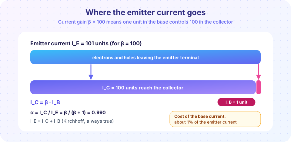
Current cannot disappear inside a transistor, so the three terminal currents (taken positive into the collector and base, out of the emitter, for an npn device) obey
I_E = I_C + I_B
Two gains describe how this total divides.
- α = I_C / I_E. For a good BJT this is 0.98 to 0.999.
- β = I_C / I_B.
Substitute I_E = I_C + I_B and the two are linked:
β = α / (1 − α) and α = β / (β + 1)
This relation is very sensitive near α = 1. If α = 0.99, then β = 0.99 / 0.01 = 99. If α improves to 0.995, β doubles to 199. That is why β varies so widely from one transistor to the next, while α looks almost the same. Datasheets often quote β as h_FE with a very wide range (for instance 100 to 300 for a common small-signal device) and engineers design circuits that do not depend on its exact value.
| β | α = β/(β+1) | I_B for I_C = 10 mA |
|---|---|---|
| 20 | 0.9524 | 500 µA |
| 50 | 0.9804 | 200 µA |
| 100 | 0.9901 | 100 µA |
| 300 | 0.9967 | 33 µA |
Where does the base current come from?
The base current has three physical contributions: holes injected from the base into the emitter, electrons that recombine in the base, and recombination in the base-emitter depletion region. The first two scale as e^(V_BE/V_T), just like the collector current, so their ratio gives a constant β. The third is a recombination current in the depletion region that scales more slowly, roughly as e^(V_BE/(2V_T)).
At low currents the slower term dominates the base current and β is small. At moderate currents β reaches its peak. At high currents, high-level injection, the Kirk effect and series resistance reduce I_C growth and β falls again. A real transistor therefore has a bell-shaped β-versus-I_C curve, and quoting a single β is only meaningful at the current where it is measured.
β also grows with temperature (typically by a few tenths of a percent per kelvin) and varies with the collector voltage through the Early effect.
The Ebers-Moll model
J. J. Ebers and J. L. Moll (1954) described the BJT as two diodes with interacting currents. In its transport form, for an npn device:
I_C = I_S (e^(V_BE/V_T) − e^(V_BC/V_T)) − (I_S/β_R)(e^(V_BC/V_T) − 1)
I_B = (I_S/β_F)(e^(V_BE/V_T) − 1) + (I_S/β_R)(e^(V_BC/V_T) − 1)
β_F is the forward current gain (the one we normally call β) and β_R the much smaller reverse gain obtained when the roles of emitter and collector are swapped. The same equations cover every region:
- Forward-active (V_BE ≈ 0.7 V, V_BC strongly negative): the exponentials in V_BC vanish and you recover
I_C = I_S e^(V_BE/V_T)andI_B = I_C / β_F. - Cutoff (both junctions reverse biased): all currents are tiny leakage currents.
- Saturation (both forward biased): the V_BC terms subtract from I_C, so I_C drops below β_F I_B, a clear sign that the transistor is out of the amplifier region.
- Reverse-active: roles swap and the gain is β_R, often 1 to 5.
Transconductance: the link to amplifiers
Differentiate the active-region law:
g_m = dI_C/dV_BE = I_C / V_T
At I_C = 1 mA this is 1e-3 / 0.02585 = 38.7 mS. A BJT with a collector resistor R_C and a small input signal v_be has a voltage gain of about −g_m R_C. With R_C = 4.7 kΩ and I_C = 1 mA, that is −38.7 mS × 4.7 kΩ ≈ −182. A bipolar amplifier therefore gets large gain from small bias currents, and g_m depends only on current and temperature, not on device geometry.
Common misconceptions
"β is a fixed property of the transistor." It changes with current, temperature and collector voltage, and varies by a factor of three between nominally identical parts. Design for the minimum β on the datasheet.
"A larger β means a better transistor in every way." High β often comes with a lower breakdown voltage and worse linearity; fast RF transistors typically have a moderate β.
"I_C = β·I_B always holds." It holds only in the forward-active region. In saturation, I_C is set by the external circuit and is smaller than β·I_B.
Try it
The Python cell builds a realistic Gummel plot from the Ebers-Moll ideas plus a recombination current and a high-injection knee. Look for the three regimes of β on the lower panel.
Press Run (or Ctrl + Enter) to see the result here.
Program input · what you'd type while the program runs
Type the answers before you press Run, one per line. Each time the program reads a line (with input()), it gets the next line from this box.
Now an interactive operating-point explorer. Move the V_BE slider: the widget computes I_C, I_B (β = 100), I_E and g_m from the exponential law. It is a calculator for the active region only and does not model saturation.
Check your understanding
Quick check · 5 questions
of 5 answered You scored / 5 · perfect!
-
1. A transistor has β = 199. What is α?
α = β/(β+1) = 199/200 = 0.995. -
2. At I_C = 2 mA and T = 300 K, the transconductance of a BJT is about
g_m = I_C/V_T = 2 mA / 25.85 mV = 77 mS. -
3. Which statement about β is true?
β has a bell-shaped dependence on I_C and rises with temperature; datasheets give a wide range. -
4. In saturation, compared with β·I_B the collector current is
The forward-biased base-collector junction subtracts from I_C, so I_C < β·I_B. The ratio I_C/I_B is the 'forced beta'. -
5. Which term in the base current dominates at very low V_BE?
The depletion-region recombination current grows as e^(V_BE/2V_T) and dominates when the main terms are still tiny.
Summary
I_E = I_C + I_B;α = I_C/I_E = β/(β+1);β = α/(1−α).- β is not constant: it varies with current, temperature and part, so circuits must tolerate a wide spread.
- Ebers-Moll uses two exponentials (the two junctions) and reduces to
I_C = I_S e^(V_BE/V_T)in the forward-active region. g_m = I_C/V_T, about 38.7 mS per milliamp at room temperature, which gives large voltage gain from small currents.
Next: Regions and switching
Track your progress
Create a free account to tick off lessons and pick up where you left off on any device.
of Semiconductor Devices lessons completed