


















Lesson 10 of 46 · Measuring Disease
Chapter 3 overview: measuring disease
Preview chapter 3: how epidemiologists count cases, turn counts into risks and rates, compare groups fairly and quantify associations, with a simulation of chance variation.
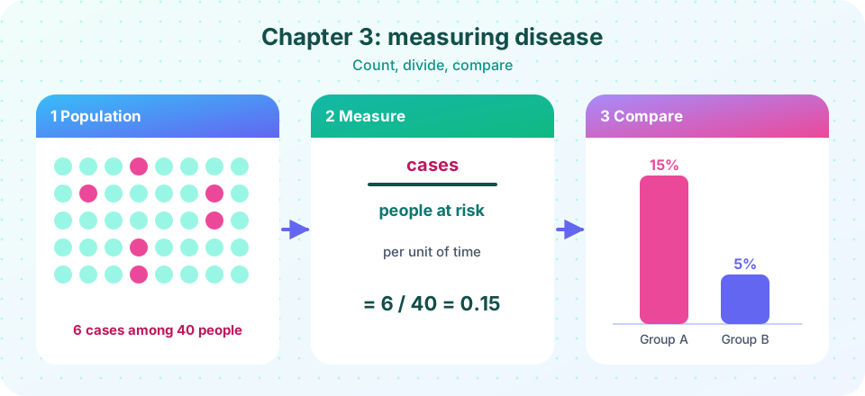
Public health decisions rest on numbers, and the numbers are only useful when they are the right numbers. How many people fell ill? Out of how many? During what time? Compared with whom? This chapter gives you the vocabulary and the arithmetic to answer those questions precisely, so that you can read a health report critically and, later, produce your own.
What you will learn
- The big picture of chapter 3 and how its four lessons connect.
- Why measures must name a numerator, a denominator and a time.
- How chance alone makes identical groups look different.
Key terms
- Measure of frequency: a number that says how common a health event is (risk, rate, prevalence).
- Measure of association: a number that compares frequencies between groups (risk ratio, odds ratio, risk difference).
- Random variation: differences between samples or places caused by chance alone.
- Standardization: adjusting rates so that groups with different age structures can be compared fairly.
The four ideas
- Count properly
- Frequency
- Compare fairly
- Associate
What each lesson covers
- Ratios, proportions and rates separates three look-alike measures, introduces person-time, and shows how an incidence rate is built from follow-up of individuals.
- Incidence and prevalence explains cumulative incidence, incidence rate and point and period prevalence, and the bathtub relationship between them.
- Mortality and standardization covers death rates, case fatality, and why age-adjusted rates are needed for fair comparison.
- Measures of association builds the two-by-two table and derives risk ratio, risk difference, odds ratio, attributable fractions and the number needed to treat.
- Chapter 3 review consolidates it all with a ten-question quiz.
A word about chance
Whenever you compare two numbers from samples or small populations, ask whether the difference could be due to chance. Even if two towns have exactly the same underlying risk, the number of cases that actually occur will vary from year to year and place to place, just as ten coin-tossing sessions of 100 tosses will not all give exactly 50 heads. This random variation matters most for small populations and rare events. The more cases there are, the more stable a rate is. Later chapters will show you how confidence intervals describe this uncertainty. For now, use the simulation below to see it with your own eyes: ten towns with an identical risk of 3 percent produce case counts that span a wide range.
Two other sources of misleading numbers will accompany us throughout the course. Bias is systematic error in how people are selected or measured. Confounding is a mixing of effects caused by a third factor. We treat both carefully in chapter 5, but you will meet them already in the measures here, for instance in the problem of comparing death rates between a young and an old town.
Notation used in this chapter
A few symbols recur, so it helps to meet them now. We write a, b, c and d for the four cells of a two-by-two table (exposed and diseased, exposed and not diseased, unexposed and diseased, unexposed and not diseased). N is the size of a population, PT stands for person-time, I for incidence and P for prevalence. When a quantity is an estimate from a sample, the text says so. Formulas are written in plain text, such as risk = cases / people at risk, and are always followed by a worked example with numbers you can recompute yourself.
Units deserve special care in this chapter. A risk is a pure number between 0 and 1 and needs a time period. A rate has units of one over time, such as per person-year. A rate ratio, risk ratio and odds ratio are pure numbers with no unit. When you meet a figure, ask which kind of number it is, and you will rarely go wrong.
Try it
Press Run (or Ctrl + Enter) to see the result here.
Program input · what you'd type while the program runs
Type the answers before you press Run, one per line. Each time the program reads a line (with input()), it gets the next line from this box.
Check your understanding
Quick check · 3 questions
of 3 answered You scored / 3 · perfect!
-
1. Which pair describes a measure of association?
Measures of association compare frequencies between groups; risk ratio and odds ratio are classic examples. -
2. Ten towns have exactly the same true risk, but observed case counts differ. The best explanation is
Even with an identical underlying risk, observed counts vary by chance, especially in small populations. -
3. Why standardize death rates?
Age strongly affects death rates, so crude rates of young and old populations are not directly comparable.
Summary
- Measures of frequency describe how common an event is; measures of association compare groups.
- Every measure needs a numerator, a denominator and a time period.
- Chance, bias and confounding can all make numbers misleading; standardization handles age.
- The next four lessons build the measurement toolkit step by step.
Track your progress
Create a free account to tick off lessons and pick up where you left off on any device.
of Public Health and Epidemiology lessons completed