


















Lesson 23 of 46 · Causation and Bias
Confounding and Association
Learn what a confounder is, the three conditions it must meet, how Simpson's paradox arises, and how matching, restriction, stratification and randomization control it.
Confounding is the most important idea in observational epidemiology, and it is also the most misunderstood. In plain language, confounding happens when the effect of the exposure you care about gets mixed up with the effect of something else. The result is that the crude comparison between exposed and unexposed people tells the wrong story, sometimes exaggerating an effect, sometimes hiding one, and occasionally even reversing it.
This lesson defines confounding precisely, shows how it can flip a result around (Simpson's paradox), and explains the standard tools for dealing with it: design choices before the study, and analysis choices afterwards.
What you will learn
- State the three conditions a variable must meet to be a confounder.
- Explain how Simpson's paradox shows confounding in numbers.
- Distinguish confounders from mediators and colliders.
- Compare control methods: randomization, restriction, matching, stratification and regression.
- Compute a stratified (Mantel-Haenszel) risk ratio from a table.
Key terms
Confounder: a factor that is associated with the exposure, is an independent cause (or marker) of the outcome, and is not on the causal pathway between them.
Stratification: analyzing the exposure-outcome link separately within levels of a third variable.
Adjusted estimate: an effect estimate that has been corrected for one or more confounders.
Residual confounding: confounding that remains because a confounder was measured badly or not at all.
Effect modification: a real difference in the exposure's effect across groups. It is something to report, not something to remove.
The three conditions
A variable is a confounder of the link between exposure E and outcome D only if all three of these hold:
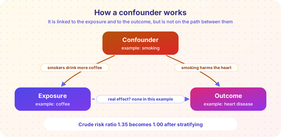
- It is associated with the exposure among the people studied (smokers drink more coffee than non-smokers).
- It is associated with the outcome independently of the exposure (smoking raises the risk of heart disease whether or not you drink coffee).
- It is not a step on the causal pathway from E to D (coffee does not make people smoke).
The third condition is easy to forget and it matters. Suppose a salt-reduction program lowers blood pressure, and lower blood pressure lowers stroke risk. Blood pressure is a mediator on the path from salt reduction to fewer strokes. If you "adjusted" for blood pressure, you would erase part of the very effect you want to measure. Adjusting for a confounder removes bias; adjusting for a mediator removes the effect.
A related trap is the collider: a variable caused by both the exposure and the outcome (or by factors related to them). Restricting your study to a collider, for example only hospital patients when both a disease and an exposure lead to admission, can create a fake association. Berkson described this in 1946, and the next lessons return to it as selection bias. Causal diagrams (directed acyclic graphs, DAGs) make these roles visible, and the causal inference track develops them further.
Confounding in numbers: Simpson's paradox
Consider the invented data below about coffee drinking and heart disease. The first row compares everyone; the next rows separate smokers from non-smokers.
| Group | Coffee drinkers (cases / people) | Non-drinkers (cases / people) | Risk ratio |
|---|---|---|---|
| Everyone | 132 / 1,900 (6.9%) | 108 / 2,100 (5.1%) | 1.35 |
| Smokers | 84 / 700 (12%) | 36 / 300 (12%) | 1.00 |
| Non-smokers | 48 / 1,200 (4%) | 72 / 1,800 (4%) | 1.00 |
Within each smoking group, coffee makes no difference at all (risk ratio 1.00). Yet the crude table shows 35% more disease among coffee drinkers. The reason is the mix of people: 37% of coffee drinkers smoke (700 of 1,900) compared with only 14% of non-drinkers (300 of 2,100), and smokers carry three times the risk. The crude comparison is partly a comparison of smokers with non-smokers.
The more dramatic version is Simpson's paradox, where the crude association goes one way and the stratified associations go the other. A frequently cited real case is the 1973 graduate admissions data from the University of California, Berkeley. Overall, men were admitted at a clearly higher rate than women (roughly 44% against 35%). Bickel, Hammel and O'Connell (1975) showed that within most individual departments women were admitted at similar or higher rates; women had applied more often to departments with low admission rates. Department confounded the comparison.
Be careful with the lesson here. Simpson's paradox does not say "always stratify". Whether the crude or the stratified answer is the right one depends on the causal structure: you must know whether the third variable is a confounder, a mediator or a collider. Statistics alone cannot tell you, which is why subject knowledge belongs in the analysis.
Controlling confounding
Some methods work at the design stage, others at the analysis stage.
At the design stage
- Randomization. In a randomized trial a coin toss decides who gets the exposure, so on average all other factors, measured or not, are balanced. This is why trials are the strongest design for causal questions (chapter 4).
- Restriction. Only include people in one level of the confounder, for example only non-smokers. It is simple and effective but reduces sample size and limits who the results apply to.
- Matching. In a case-control study, pick controls with the same age and sex as cases. Matching ensures balance on those factors, but a matched design must then be analyzed as matched, and you cannot study the matching variable itself.
At the analysis stage
- Stratification. Compute the effect within each stratum and then combine them. The Mantel-Haenszel estimate gives a weighted average of the stratum-specific risk ratios (or odds ratios). For risk ratios, with
aexposed cases,n1exposed people,cunexposed cases,n0unexposed people, andNtotal in a stratum:
RR_MH = sum(a * n0 / N) / sum(c * n1 / N)
- Standardization. Compare rates after weighting each group to a common age structure (you met this in chapter 3).
- Multivariable regression. Logistic, Poisson or Cox models estimate the exposure's effect while holding other measured variables fixed. Regression handles many confounders at once but can only adjust for what was measured.
For the table above, the stratified calculation is (84*300/1000 + 48*1800/3000) / (36*700/1000 + 72*1200/3000) which is (25.2 + 28.8) / (25.2 + 28.8) = 1.00. The confounded crude ratio of 1.35 disappears.
Residual confounding and what we can never fully rule out
No adjustment is perfect. Residual confounding remains when the confounder is measured crudely ("ever smoked" instead of pack-years), or when it was not measured at all. Epidemiologists therefore ask a specific question about every observational result: what confounders might remain, and how strong would they need to be to explain the finding? A sensitivity technique called the E-value (VanderWeele and Ding, 2017) puts a number on that: it states how strongly an unmeasured confounder would have to be related to both exposure and outcome to fully explain the observed association.
Modern studies also use designs that approximate randomization, such as natural experiments and Mendelian randomization (using genetic variants as proxies for exposures). They are powerful, yet each comes with assumptions of its own.
Common misconceptions
"Adjusting for everything you can measure is always better." Adjusting for mediators or colliders can introduce bias. Choose adjustment variables using subject knowledge, ideally a causal diagram.
"Confounding means the result is wrong." It means the crude result is misleading. Handled well, the adjusted result may be fine.
"If the sample is big, confounding disappears." Confounding is a bias, and bias does not shrink with sample size.
Try it
This simulation reproduces the numbers from the table above and computes the crude and the Mantel-Haenszel risk ratios. Edit the counts to see how strongly the stratified answer depends on them.
Press Run (or Ctrl + Enter) to see the result here.
Program input · what you'd type while the program runs
Type the answers before you press Run, one per line. Each time the program reads a line (with input()), it gets the next line from this box.
Now explore the same idea by hand. Toggle between the combined table and the two strata, and watch the apparent effect appear and vanish.
Check your understanding
Quick check · 5 questions
of 5 answered You scored / 5 · perfect!
-
1. Which condition must a confounder NOT meet?
A variable on the causal pathway is a mediator. Adjusting for it removes part of the real effect. -
2. Which design method balances measured AND unmeasured factors on average?
Random allocation balances all factors, known or unknown, in expectation. The other methods handle only chosen factors. -
3. In the Berkeley admissions example, what played the role of the confounding variable?
Women applied more to departments with lower admission rates, so department was linked to both sex and admission. -
4. A crude risk ratio is 1.35 and the Mantel-Haenszel risk ratio is 1.00. What is the best interpretation?
When stratifying removes the association, the stratifying variable was confounding the crude comparison. -
5. Why is it risky to adjust for a mediator?
The mediator carries some of the effect, so controlling for it hides that part.
Summary
- A confounder is linked to the exposure, independently affects the outcome and is not on the causal pathway.
- Simpson's paradox shows that crude and stratified results can disagree, so the causal structure must guide the analysis.
- Randomization, restriction and matching act at the design stage; stratification, standardization and regression act at the analysis stage.
- Residual confounding always remains a possibility, and sensitivity analyses such as the E-value help judge it.
Track your progress
Create a free account to tick off lessons and pick up where you left off on any device.
of Public Health and Epidemiology lessons completed