


















Lesson 18 of 46 · Study Designs
Cohort studies: following exposed and unexposed people forward in time
Understand prospective and retrospective cohort studies, landmark examples such as Framingham and the British Doctors Study, person-time analysis and the problem of loss to follow-up.
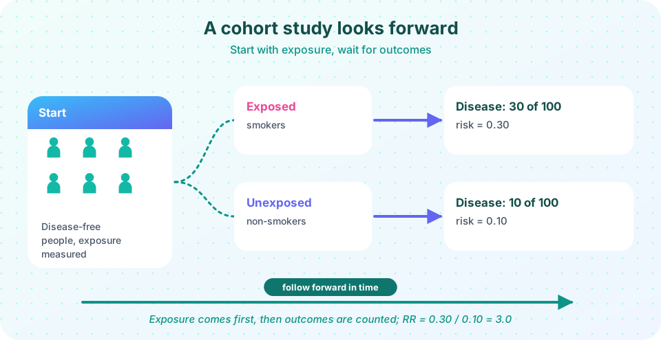
If you suspect that smoking causes lung cancer, a natural way to find out is to gather a large group of people, record who smokes and who does not, and then wait to see who develops cancer. That is a cohort study. The word cohort comes from the Roman army, where a cohort was a unit of soldiers; in epidemiology it means a group of people who share some characteristic and who are followed over time.
Cohort studies are the workhorse of research on long-term risk factors. They produced our knowledge of the links between smoking and cancer, blood pressure and stroke, diet and heart disease. This lesson explains how they are built, how to analyze them, what they do well and where they can go wrong.
What you will learn
- How a cohort study is designed and what makes it prospective or retrospective.
- Landmark cohorts: Framingham, the British Doctors Study and the Nurses' Health Study.
- How to analyze a cohort with risks, rates and survival curves.
- Strengths and weaknesses, including loss to follow-up.
Key terms
- Cohort: a group of people followed over time.
- Prospective cohort: exposure is measured now and outcomes are observed in the future.
- Retrospective (historical) cohort: both exposure and outcome have already occurred, and records are used to reconstruct the follow-up.
- Loss to follow-up: participants who leave the study before outcomes are known.
- Healthy worker effect: workers tend to be healthier than the general population, which can bias occupational studies.
How a cohort study works
- Choose a population that is free of the outcome at the start. For a question about lung cancer, enroll people without lung cancer.
- Measure exposure at baseline (for example, smoking habits, blood pressure, diet) and, ideally, again over time.
- Follow everyone for a defined period, watching for the outcome. Use registries, repeat examinations, questionnaires or medical records.
- Compare the occurrence of the outcome in the exposed group with that in the unexposed group, using risk ratios, rate ratios or hazard ratios.
Because exposure is recorded before the outcome occurs, a cohort study establishes temporality: the exposure came first, which is a necessary condition for causation. It also allows you to compute actual incidence, risks and rates, in contrast to case-control studies, and to study several outcomes from a single exposure (smoking and lung cancer, heart disease, stroke, chronic bronchitis).
Prospective and retrospective cohorts
In a prospective cohort, the investigators enroll people now and wait. This gives the best control over how exposures are measured, but can take years and be costly. In a retrospective (or historical) cohort, the investigators go back to existing records. For example, they might use employment files of a chemical plant from 1960, identify who worked with a solvent, and then check death records through 2020. Both exposure and outcome have already happened, but the logic is still forward in time: from exposure to outcome. The advantages are speed and cost, and the main weakness is dependence on whatever data were recorded. Some studies combine both (ambispective).
Landmark cohorts
The Framingham Heart Study began in 1948 in Framingham, Massachusetts, with about 5,200 adults aged 30 to 62 who were examined every two years. It has since included their children and grandchildren. Framingham established that high blood pressure, high cholesterol, smoking, obesity and diabetes increase the risk of heart disease, and the term risk factor itself was popularized by its investigators in the early 1960s. Its data underlie risk calculators used in clinics.
The British Doctors Study began in 1951 when Richard Doll and Austin Bradford Hill, who had previously reported a case-control study of smoking and lung cancer, asked all doctors on the British Medical Register to describe their smoking habits, and followed more than 30,000 male doctors. Within a few years the lung cancer death rate was clearly rising with the amount smoked. A report after 50 years found that lifelong smokers lost on average about ten years of life compared with non-smokers, and that quitting, even at middle age, reduced the loss. Doctors were a convenient group: easy to contact and follow, with good health records, and similar education, which reduced some confounding.
The Nurses' Health Study, begun in 1976 by researchers at Harvard, enrolled about 120,000 female nurses and followed them with regular questionnaires on diet, medications and health. It produced evidence on hormone therapy, diet, smoking and many other topics, and also provided a famous example of how observational findings can conflict with later trials: early cohort results suggested that hormone therapy protected women against heart disease, but randomized trials later found no such protection, a discrepancy usually attributed to confounding and bias in the observational data (chapter 5).
Analyzing a cohort
If everyone is followed for the same period and nobody is lost, you can compute risk in each group and the risk ratio and risk difference, as in the previous lesson. With unequal follow-up, use person-time and compare incidence rates. The first demonstration simulates a cohort of 4,000 people, 30 percent exposed, in which the true effect of exposure is to double the event rate. By counting events and person-years, the analysis recovers a rate ratio close to two with a confidence interval around it. The simulated data also include random loss to follow-up, which the person-time method handles.
A common display is the cumulative incidence (or Kaplan-Meier) curve, which shows the proportion who have had the event by each time. A widening gap between exposed and unexposed curves indicates an effect. Longer analyses use Cox proportional hazards regression, which reports a hazard ratio and can adjust for confounding variables, a topic that returns in chapter 5.
Strengths and weaknesses
Strengths
- Temporal sequence is clear: exposure comes before outcome.
- Direct estimates of incidence, risk and rate.
- Several outcomes can be studied for one exposure.
- Good for rare exposures (for example, a cohort of workers exposed to a rare chemical).
- Exposure can be measured before disease develops, avoiding recall bias.
Weaknesses
- Costly and slow, particularly for diseases with long latency.
- Inefficient for rare diseases: you need huge numbers of people to see enough cases.
- Loss to follow-up can bias results, especially if it differs between groups or is related to the outcome.
- Exposure may change over time (people stop smoking), so a single baseline measurement misclassifies.
- Confounding remains a problem because exposure is not randomized: smokers also differ from non-smokers in diet, alcohol and other ways.
- Selection effects such as the healthy worker effect and the "healthy volunteer" effect make cohorts unrepresentative.
Loss to follow-up in numbers
Suppose a cohort has 1,000 exposed and 1,000 unexposed people, with 100 and 50 cases respectively: a true risk ratio of 2.0. Now suppose that, among those who develop the disease, 40 percent of the exposed are lost to follow-up and never counted (perhaps they became too sick to attend), compared with 10 percent of the unexposed. The observed cases are 60 and 45, and the apparent risk ratio falls to 1.33. The study underestimates the association, because the losses were related to both exposure and outcome. The second demonstration runs this calculation. That is why cohort studies report how many were lost and try to follow up everyone through registries, and why analysts examine whether those lost differ from those retained.
Common misconceptions
"Cohort studies prove causation." They provide good evidence of temporal order and incidence, but without randomization, confounding and bias remain possible.
"Prospective always means better." A well-run retrospective cohort with excellent records can be more reliable than a poorly run prospective one.
"A cohort study can only study one outcome." One of its advantages is the ability to examine several outcomes of the same exposure.
"Loss to follow-up only reduces sample size." It can also bias results if those lost differ from those who remain, particularly in a way related to exposure and outcome.
Try it
Press Run (or Ctrl + Enter) to see the result here.
Program input · what you'd type while the program runs
Type the answers before you press Run, one per line. Each time the program reads a line (with input()), it gets the next line from this box.
Press Run (or Ctrl + Enter) to see the result here.
Program input · what you'd type while the program runs
Type the answers before you press Run, one per line. Each time the program reads a line (with input()), it gets the next line from this box.
Check your understanding
Quick check · 6 questions
of 6 answered You scored / 6 · perfect!
-
1. What is the key difference between prospective and retrospective cohort studies?
In a prospective cohort, exposure is measured now and outcomes are awaited. In a retrospective cohort, both have already occurred and records are used. -
2. Which is a strength of a cohort study?
Temporality and direct incidence estimates are core strengths; cost and efficiency for rare outcomes are weaknesses. -
3. A cohort has 40 cases among 1,000 exposed and 10 among 1,000 unexposed. The risk ratio is
0.04 / 0.01 = 4. -
4. Why can differential loss to follow-up bias a cohort study?
Losses that are related to both exposure and outcome change the observed ratio. -
5. The British Doctors Study mainly demonstrated
Doll and Hill's cohort showed rising mortality with smoking and benefits of quitting. -
6. Which situation is best suited to a cohort design?
Cohorts follow exposed groups, so they are efficient when the exposure is rare.
Summary
- A cohort study follows people from exposure to outcome, so temporality is clear and incidence can be measured.
- Cohorts can be prospective or retrospective; Framingham, the British Doctors Study and the Nurses' Health Study are landmark examples.
- Analyze with risks, person-time rates or survival curves; losses to follow-up can bias results.
- Cohorts are costly and inefficient for rare outcomes, and remain open to confounding because exposure is not randomized.
Next: Case-control studies
Track your progress
Create a free account to tick off lessons and pick up where you left off on any device.
of Public Health and Epidemiology lessons completed