


















Lesson 45 of 46 · Projects and Practice
Epidemiology Cheat Sheet: Formulas and Checklists
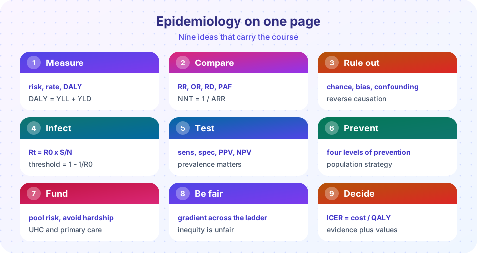
A one-page epidemiology recap: core formulas for risk, odds, screening, infection and economics, a bias checklist, a causal reasoning routine and a reusable Python function library.
This page is a quick reference for the second half of the course. It will not replace the lessons, but it puts the formulas, the questions to ask and the traps to avoid in one place, so you can review before an exam or while reading a paper.
What you will learn
- Recall the core formulas of chapters 5 to 8 in one place.
- Use a checklist to appraise a study for bias and confounding.
- Reuse a small set of Python functions for common calculations.
Key terms
RR, OR, RD: risk ratio, odds ratio and risk difference.
PAF: population attributable fraction.
R0 and Rt: basic and effective reproduction numbers.
PPV and NPV: predictive values of a test.
ICER: cost per extra QALY.
Core formulas
| Area | Formula |
|---|---|
| Risk ratio | RR = risk(exposed) / risk(unexposed) |
| Risk difference | RD = risk(exposed) - risk(unexposed) |
| Odds ratio (2x2: a, b, c, d) | OR = (a x d) / (b x c) |
| CI for ln(OR) | ln(OR) +/- 1.96 x sqrt(1/a + 1/b + 1/c + 1/d) |
| Mantel-Haenszel RR | sum(a x n0 / N) / sum(c x n1 / N) |
| Attributable fraction (exposed) | (RR - 1) / RR |
| PAF | p(RR - 1) / (1 + p(RR - 1)) |
| ARR and NNT | ARR = control risk - treated risk; NNT = 1 / ARR |
| Sensitivity, specificity | TP/(TP+FN); TN/(TN+FP) |
| PPV, NPV | TP/(TP+FP); TN/(TN+FN) |
| Likelihood ratio | LR+ = Sens/(1 - Spec); post-test odds = pre-test odds x LR |
| Doubling time | ln 2 / r |
| R0 from growth | about 1 + r x T_g |
| SIR | R0 = beta / gamma; Rt = R0 x S/N |
| Herd immunity | 1 - 1/R0; coverage = (1 - 1/R0) / efficacy |
| Vaccine efficacy | 1 - RR |
| DALY | YLL + YLD |
| ICER | extra cost / extra QALYs |
The bias and confounding checklist
When you read a study, ask these questions in order.
- Chance: how big is the sample, and what is the confidence interval?
- Selection: who was included, who refused, who dropped out? Were controls from the source population?
- Information: how were exposure and outcome measured, and could errors differ between groups?
- Confounding: what else could explain the link? Was it measured, and was it adjusted for correctly (not a mediator or a collider)?
- Reverse causation: could the outcome have changed the exposure?
- Strength and dose-response: is the effect large, and does it increase with dose?
- Consistency and plausibility: do other studies agree, and is there a mechanism?
- Experiment: does removing the exposure reduce disease?
- Consequences: how costly is it to be wrong, and how big is the absolute effect?
Study-design quick guide
| Design | Starts with | Gives | Typical weaknesses |
|---|---|---|---|
| Randomized trial | Assigned exposure | RR, RD | Cost, ethics, generalizability |
| Cohort | Exposure groups | Incidence, RR | Loss to follow-up, confounding |
| Case-control | Cases and controls | OR | Recall bias, control selection |
| Cross-sectional | A snapshot | Prevalence | Cannot show time order |
| Ecological | Group data | Group correlations | Ecological fallacy |
Infection, chronic disease and policy in one line each
- Infection: break the chain; keep Rt below 1; investigate with person-place-time and attack rates; vaccinate above the threshold.
- Chronic disease: many causes and long latency; relative risks show strength, absolute risks show impact; screening can mislead through prevalence and bias; population strategies reach the moderate-risk majority.
- Systems and policy: six building blocks; pooling protects; the social gradient runs across the whole ladder; evaluate policies with designs that handle trends; compare interventions by ICER and equity.
Worked mini-examples to anchor the formulas
- Odds ratio: exposed cases 40, unexposed cases 60, exposed controls 25, unexposed controls 75. OR = (40 x 75) / (60 x 25) = 3000 / 1500 = 2.0.
- PAF: 25% exposed, RR = 3. PAF = 0.25 x 2 / (1 + 0.25 x 2) = 0.5 / 1.5 = 33%.
- Screening: 1,000 people, prevalence 2%, sensitivity 90%, specificity 90%. Diseased 20: TP 18, FN 2. Healthy 980: FP 98, TN 882. PPV = 18 / 116 = 15.5%.
- Herd immunity: R0 = 3 gives a threshold of 67%; with a vaccine that is 80% effective the coverage needed is 0.667 / 0.8 = 83%.
- NNT: risk falls from 6% to 4.5%. ARR = 1.5 points, NNT = 1 / 0.015 = 67.
- ICER: extra cost 9,000 for 0.3 extra QALYs gives 30,000 per QALY.
Rules of thumb for interpreting numbers
- A relative risk below about 1.5 or above about 0.67 from an observational study is easily produced by modest bias or confounding, so treat it with caution unless it is very consistent.
- A confidence interval shows the range of values compatible with the data under the study's assumptions. A narrow interval around a biased estimate is still biased.
- P-values measure how surprising the data would be if there were no effect; they do not give the probability that the hypothesis is true and do not measure the size of an effect.
- Absolute risk matters for decisions. Multiply the baseline risk by the relative risk and compare.
- For a rare disease the odds ratio and the risk ratio are almost the same; for a common outcome the odds ratio is farther from 1.
- Positive predictive value is low when the disease is rare, even for a good test. Ask what prevalence applies to the person in front of you.
- R0 above 1 means growth; Rt below 1 means decline. Control measures aim to push Rt under 1, and the required reduction is 1 - 1/R0.
- Doubling time gives a quick feel for growth: 7 days means about 10% per day, and 3 days means about 26% per day.
- Every policy has trade-offs. State who benefits, who pays and what is unknown.
Five questions to ask of any health headline
- What was the comparison, and who were the people?
- What is the absolute risk, not only the relative change?
- Could something else explain the link (confounding, bias, reverse causation)?
- Does it agree with other studies and with biology?
- What would change if it were true, and what would it cost to be wrong?
Try it
A reusable Python function library for the formulas above. Copy it into your own work and call the functions with your own numbers. The demo at the end exercises each one.
Press Run (or Ctrl + Enter) to see the result here.
Program input · what you'd type while the program runs
Type the answers before you press Run, one per line. Each time the program reads a line (with input()), it gets the next line from this box.
Second, a bias-and-confounding appraisal checklist for a study you are reading. Tick the questions you can answer well; the tool lists what is left to check.
Check your understanding
Quick check · 4 questions
of 4 answered You scored / 4 · perfect!
-
1. Which formula gives the population attributable fraction?
The middle formula is the attributable fraction among the exposed, and the last gives the NNT. -
2. Which design is most affected by recall bias?
Cases and controls report past exposures after the outcome is known. -
3. The herd immunity coverage needed with R0 = 4 and efficacy 0.9 is closest to:
(1 - 0.25) / 0.9 = 0.833. -
4. In the checklist, what is the correct order of the first four questions?
The routine goes from the role of luck to design problems in who and how, then to confounders.
Summary
- Keep the formulas for risk, odds, attributable fractions, screening, infection and economics at hand.
- Appraise any study for chance, selection, information, confounding and reverse causation before judging cause.
- Match each design to its typical weaknesses.
- Reuse the Python function library for your own calculations.
Next: Further study
Track your progress
Create a free account to tick off lessons and pick up where you left off on any device.
of Public Health and Epidemiology lessons completed