


















Lesson 27 of 45 · Control and Modulation
PWM and sinusoidal PWM
Learn how a carrier and a reference make PWM: duty cycle, modulation index, frequency ratio, harmonics, unipolar and bipolar switching, third-harmonic injection and dead-time errors.
In the previous chapter the inverter switched its legs once per cycle, producing square waves and six-step staircases. That is simple, but the harmonics are large and the amplitude cannot be adjusted without changing the DC link. Pulse-width modulation (PWM) solves both problems by switching many times per output cycle and varying the width of each pulse. The average voltage over each switching period then follows a reference that you choose, for example a sine wave of any amplitude and frequency.
This lesson shows how a PWM modulator works, how to measure its performance with two numbers (ma and mf), where the harmonics end up, and what limits the output voltage.
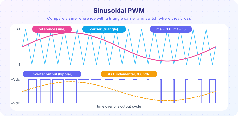
What you will learn
- Generate PWM by comparing a reference with a carrier and compute the duty cycle.
- Define and use the modulation index
maand frequency ratiomf. - Locate the harmonics of sinusoidal PWM and compare bipolar and unipolar switching.
- Use third-harmonic injection to gain 15 % more output voltage.
- Explain how dead time distorts the output and how digital PWM resolution limits it.
Key terms
Carrier: the triangle or sawtooth wave, at the switching frequency, that the reference is compared with.
Modulation index (ma): reference amplitude divided by carrier amplitude, ma = V̂ref / V̂carrier.
Frequency modulation ratio (mf): switching frequency divided by output frequency, mf = fsw / f1.
Overmodulation: operation with ma > 1, where pulses merge and low-order harmonics appear.
Third-harmonic injection: adding a small third harmonic to the reference to extend the linear range.
How PWM is generated
Take a reference signal vref (a constant for a DC-DC converter, a sine for an inverter) and a carrier vcar with peak value V̂car at the switching frequency. The comparator output is high whenever vref > vcar. For a triangle carrier the pulses are centered in each period (symmetrical PWM); a sawtooth carrier gives pulses that start or end at the period boundary. Triangle carriers are preferred for inverters because the harmonics are smaller and the current sample at the pulse center is clean.
If vref is constant, the duty cycle is d = (vref + V̂car) / (2·V̂car) for a bipolar triangle (−V̂car … +V̂car) and the leg's pole voltage averages Vdc·d. In a DC-DC converter the same idea is used with a unipolar ramp, giving d = vc / Vramp.
In a digital controller the carrier is a counter. A timer counts from 0 to N and the compare register decides where the output toggles. The resolution is N = fclk / fsw steps per period: at fclk = 100 MHz and fsw = 100 kHz you get 1,000 steps (about 10 bits), so the smallest duty change is 0.1 %. Higher switching frequency means coarser duty resolution, a real limit when regulating a voltage to a fraction of a percent.
Modulation index and frequency ratio
For sinusoidal PWM the reference is vref = ma·V̂car·sin(2π f1 t). Two numbers describe the operation:
ma = V̂ref / V̂car          (modulation index)
mf = fsw / f1              (frequency modulation ratio)
In the linear range, ma ≤ 1, the fundamental of the output is exactly proportional to ma:
single-phase bipolar full bridge:   V1 = ma · Vdc
three-phase leg (pole voltage):     V̂an,1 = ma · Vdc / 2
three-phase line-line (rms):        VLL,1 = (√3 / (2√2)) · ma · Vdc = 0.612 · ma · Vdc
Compare these numbers with the six-step inverter's 0.780 Vdc: sinusoidal PWM reaches at most 78.5 % of the six-step fundamental, because the carrier takes its share. That is the price of the cleaner waveform.
If ma > 1 the reference exceeds the carrier peak for part of the cycle: the pulses merge, the output grows more slowly than ma and low-order harmonics (5th, 7th) appear. As ma → ∞ the waveform tends to the six-step wave.
Where the harmonics go
The great advantage of PWM is that the harmonics are not at 3f1, 5f1, 7f1 but are pushed up to the switching frequency. For a bipolar full bridge (output ±Vdc):
- The harmonics cluster around
mf, 2mf, 3mf, …with sidebands spaced by2·f1:mf ± 2,mf ± 4and so on. The strongest is nearmf. - For
mfodd and an integer, the waveform has half-wave symmetry and there are no even harmonics. Choosemfodd and, for three-phase, a multiple of 3 so that triplen harmonics cancel in the line voltages. - When
mfis small (below about 21) keep the carrier synchronized to the reference; otherwise subharmonics appear. For largemfthe carrier can run asynchronously.
Unipolar switching drives each leg of the full bridge with its own reference (+vref and −vref) so the output can step through +Vdc, 0, −Vdc. The effective ripple frequency doubles, the voltage steps are half as large and the harmonic clusters appear around 2mf, so the output filter can be about half as large. Switching losses are the same per leg.
A filter at the output (an LC low-pass with a corner well below fsw and well above f1) then removes the clusters, leaving a clean sine. This is what a grid inverter or a UPS does.
Third-harmonic injection
In a three-phase system with an isolated neutral, a common-mode term added to all three references cancels in the line-to-line voltages. Add a third harmonic of amplitude one sixth of the fundamental:
vref,a = ma · [ sin(ωt) + (1/6)·sin(3ωt) ]
The sum has a flatter top: its peak is (√3/2) = 0.866 of the fundamental amplitude. The reference can therefore be raised until its fundamental reaches 2/√3 = 1.1547 before touching the carrier. The linear range extends from ma = 1 to ma = 1.1547, a gain of 15.47 % in output voltage from the same DC link, and the maximum line-line fundamental becomes 0.612 × 1.1547 = 0.707 Vdc. Space-vector modulation (SVPWM) is the same idea in disguise: its reference is the sine plus a common-mode term equal to the average of the largest and smallest phase.
Most commercial drives use SVPWM or third-harmonic injection: it uses the DC link 15 % better than plain SPWM, with no extra hardware and a lower current ripple.
Dead time distortion
You met dead time in the previous chapter: both switches of a leg are off for a short time td. During that time the output follows the current, not the command. For a positive current the lower diode conducts and the output sits low; for a negative current it sits high. On average the leg loses a voltage of about
ΔV ≈ Vdc · td · fsw · sign(i) per leg
With Vdc = 540 V, td = 2 µs and fsw = 10 kHz this is 540 × 2e-6 × 1e4 = 10.8 V, a constant error that flips sign whenever the current crosses zero. For a drive running at low speed (small reference voltage) this error is a large fraction of the wanted voltage and causes a distorted, notchy current; controllers compensate by adding td·fsw·Vdc·sign(i) to the reference.
Common misconceptions
"A higher switching frequency is always better." It moves harmonics away and shrinks the filter, but switching losses grow in proportion to fsw, and dead time costs more voltage.
"Raising ma above 1 gives free voltage." The extra voltage costs low-order harmonics, which a motor feels as extra heating and torque ripple.
"PWM has no harmonics." It has the same total harmonic energy, but at much higher frequencies where filters and the load's inductance handle it easily.
Try it
The first example simulates single-phase bipolar sinusoidal PWM with ma = 0.8 and mf = 21, then lists the fundamental and the largest harmonics. It is a numerical simulation of ideal switching.
Press Run (or Ctrl + Enter) to see the result here.
Program input · what you'd type while the program runs
Type the answers before you press Run, one per line. Each time the program reads a line (with input()), it gets the next line from this box.
The second example compares plain sinusoidal PWM with third-harmonic injection for a three-phase leg set (mf = 45). For each modulation index it measures the fundamental line-line rms voltage. The plain curve saturates at ma = 1; the injected curve stays linear up to ma = 1.155.
Press Run (or Ctrl + Enter) to see the result here.
Program input · what you'd type while the program runs
Type the answers before you press Run, one per line. Each time the program reads a line (with input()), it gets the next line from this box.
The third example is a PWM visualizer. Change the modulation index and the carrier ratio to see where the pulses form, and watch the output reach the overmodulation region above 1. It draws the ideal comparator output.
Check your understanding
Quick check · 5 questions
of 5 answered You scored / 5 · perfect!
-
1. A three-phase SPWM inverter runs from Vdc = 600 V at ma = 0.9. What is the fundamental line-line rms output?
0.612 × 0.9 × 600 = 330 V. -
2. An inverter makes 50 Hz output with a 10 kHz carrier. What is mf?
mf = 10,000 / 50 = 200. -
3. What does third-harmonic injection achieve in a three-phase inverter?
The flat-topped reference allows ma up to 2/√3 = 1.1547 in the linear range. -
4. Dead time of 1 µs at 20 kHz switching on a 400 V link causes a per-leg average voltage error of about
ΔV ≈ Vdc·td·fsw = 400 × 1e-6 × 20,000 = 8 V. -
5. Where do the strongest harmonics of bipolar SPWM appear?
Sinusoidal PWM moves the harmonic energy up to the carrier frequency and its multiples.
Summary
- PWM compares a reference with a carrier; the duty cycle follows the reference and the average output follows it too.
ma = V̂ref/V̂carsets the amplitude (linear forma ≤ 1);mf = fsw/f1sets where the harmonics are.- Three-phase SPWM gives
VLL,1 = 0.612·ma·Vdc; third-harmonic injection or SVPWM extends the linear range toma = 1.155and0.707·Vdc. - Harmonics cluster around
mf, 2mf, …; unipolar switching doubles the effective ripple frequency. - Dead time causes an error of about
Vdc·td·fsw, which matters most at low output voltage.
Track your progress
Create a free account to tick off lessons and pick up where you left off on any device.
of Power Electronics lessons completed