


















Lesson 17 of 46 · Portfolio Theory
Two-asset portfolios: how correlation bends the curve
Work through a stock and bond portfolio by hand: expected return, volatility, the minimum-variance mix and how correlation bends the risk-return curve, with live code.
The simplest portfolio is a mix of two assets, and it contains the whole story of diversification. Everything in portfolio theory for ten assets is a larger version of what happens here. Because the algebra is small, you can follow every number, see where the curve comes from and find the mix with the least possible risk. We use an example of a stock fund and a bond fund with plain, invented figures.
What you will learn
- How to compute the expected return and volatility of any stock and bond mix.
- Why correlation determines how far the curve bends.
- How to find the minimum-variance portfolio, and why it can beat the safer asset alone.
- Which part of the curve is worth considering.
Key terms
Weight (w): the fraction of money in the first asset; the other asset gets 1 - w.
Minimum-variance portfolio: the mix with the lowest possible volatility.
Covariance: ρ × σA × σB; the term that couples the two assets.
Dominated portfolio: a portfolio with a better alternative offering more return for the same risk.
The setup
Our two assets:
| Expected return | Volatility | |
|---|---|---|
| Stocks (A) | 8% | 18% |
| Bonds (B) | 3% | 6% |
Let w be the weight of stocks and 1 - w the weight of bonds. The two quantities of interest are:
E(R) = w × 8% + (1 - w) × 3%
σ    = √( (w × 18)² + ((1 - w) × 6)² + 2 × w × (1 - w) × ρ × 18 × 6 )
The return is a straight line in w: every extra 10% moved from bonds into stocks adds 0.5 percentage points. The volatility is the interesting part, since ρ appears in it.
A worked example: 60/40
Take 60% stocks, 40% bonds with a correlation of 0.2.
- Expected return: 0.6 × 8 + 0.4 × 3 = 4.8 + 1.2 = 6.0%.
- Variance terms: (0.6 × 18)² = 10.8² = 116.64; (0.4 × 6)² = 2.4² = 5.76; cross term: 2 × 0.6 × 0.4 = 0.48, and 0.2 × 18 × 6 = 21.6, so the cross term is 0.48 × 21.6 = 10.368.
- Total variance: 116.64 + 5.76 + 10.368 = 132.768, so volatility = √132.768 ≈ 11.5%.
The weighted average of the two volatilities is 0.6 × 18 + 0.4 × 6 = 13.2%. The actual portfolio volatility, 11.5%, is lower, a gain of about 1.7 percentage points from correlation below one.
How correlation bends the curve
Try three values of ρ for the same 60/40 mix:
| ρ | Volatility of 60/40 |
|---|---|
| +1.0 | 13.2% |
| +0.2 | about 11.5% |
| -0.5 | about 9.8% |
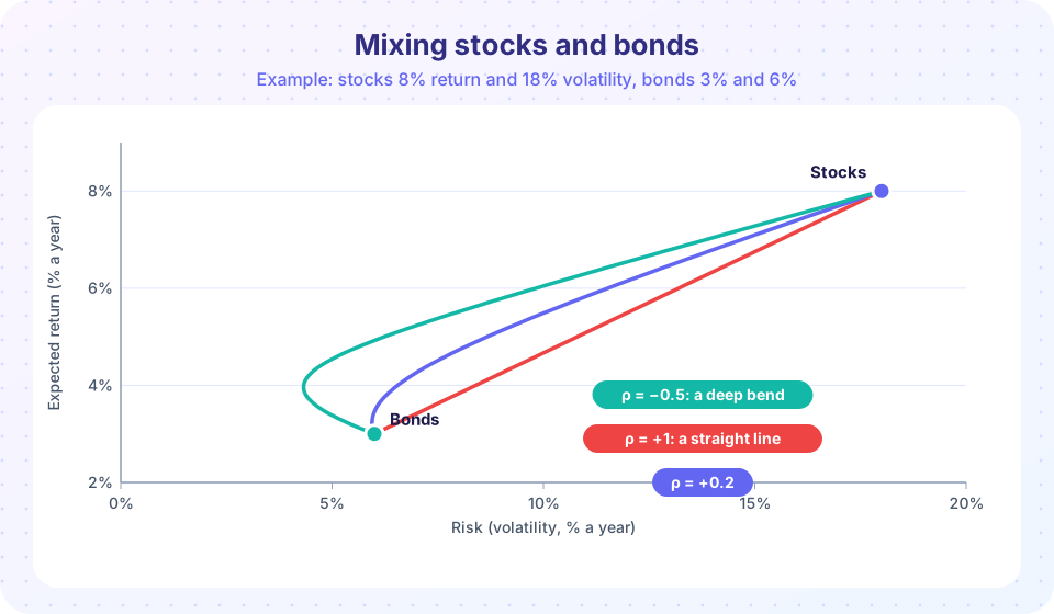
The expected return is 6.0% each time. Only the risk changes, which is exactly what the picture shows: all curves run from the bond point (lower left) to the stock point (upper right), but the lower the correlation, the further the curve bows to the left. At ρ = +1 the "curve" is a straight line, the weighted average. At ρ = -1 it would hit the vertical axis at some mix, where the portfolio's volatility is zero. For our assets that mix has w = σB / (σA + σB) = 6 / 24 = 25% in stocks. A perfect hedge like that does not exist in real markets, but it shows the limit.
The minimum-variance portfolio
Notice that the bowed curves reach a leftmost point, and then bend back to the right toward the bond point. That leftmost point is the minimum-variance portfolio: the least risky mix possible. Calculus gives a closed form for the stock weight:
w* = (σB² - ρσAσB) / (σA² + σB² - 2ρσAσB)
For ρ = 0.2: numerator 36 - 21.6 = 14.4; denominator 324 + 36 - 43.2 = 316.8; so w* = 0.0455, about 4.5% stocks. At that mix the volatility is about 5.95%, which is slightly lower than that of 100% bonds (6%). Adding a little of the riskier asset reduced risk. This surprising result is purely a correlation effect: the stock holding is small, so it contributes little risk of its own, but because it does not move in lockstep with bonds it cancels some of the bond fluctuations.
For ρ = -0.5 the same formula gives w* ≈ 19.2% in stocks and a minimum volatility of about 4.3%, far below that of either asset alone.
Which part of the curve matters?
Look at the ρ = 0.2 curve. Between the minimum-variance point and the bond point, the curve goes backward: with more bonds, you get less return and more risk. Any mix on that lower branch is dominated: moving up the curve to the minimum-variance point gives you more return for less risk. A rational investor who only cares about return and volatility never chooses the lower branch. The portfolios from the minimum-variance point up to the stock point form the efficient frontier for these two assets, the subject of the next lesson. (Mixes with w above 100%, borrowing to buy more stocks, extend the curve further up and right.)
Using the idea
For real investors, the two-asset model is a practical guide to how mixes behave. A few lessons carry over:
- Moving from 0% to 20% stocks adds much more return than risk. Because the curve starts steeply, a small stock slice does a lot for a bond-heavy portfolio.
- The curve flattens at high stock weights. The last 20% in stocks adds more risk than return.
- Correlation is an input you must estimate. It moves with time. Bond and stock correlation has been positive in some periods and negative in others, so a design that relies on a fixed negative number can disappoint.
Common misconceptions
"The minimum-risk portfolio is all in the safest asset." Not necessarily: a small slice of a riskier, imperfectly correlated asset can reduce total risk, as the 4.5% example shows.
"Portfolio volatility is the average of the volatilities." That holds only when ρ = +1.
"Negative correlation is required." Any correlation below +1 produces a benefit, and the lower, the bigger.
Try it
First, a calculator for any weight and correlation. Reproduce the 60/40 numbers and find the minimum-variance weights yourself.
Press Run (or Ctrl + Enter) to see the result here.
Program input · what you'd type while the program runs
Type the answers before you press Run, one per line. Each time the program reads a line (with input()), it gets the next line from this box.
Second, the curves from the picture, drawn from the formula. Change muA, sA or the correlations and watch the bow move.
Press Run (or Ctrl + Enter) to see the result here.
Program input · what you'd type while the program runs
Type the answers before you press Run, one per line. Each time the program reads a line (with input()), it gets the next line from this box.
Check your understanding
Quick check · 5 questions
of 5 answered You scored / 5 · perfect!
-
1. A 50/50 mix of stocks (8%) and bonds (3%) has what expected return?
0.5 × 8 + 0.5 × 3 = 5.5%. Expected return is the weighted average. -
2. When does portfolio volatility equal the weighted average of the two volatilities?
At ρ = +1 the cross term makes the formula collapse to wσA + (1-w)σB. -
3. Why can adding a little stock to an all-bond portfolio reduce its volatility?
With correlation below one, the combination can have less risk than the safer asset alone. -
4. On the curve, what is a dominated portfolio?
The lower branch below the minimum-variance point is dominated. -
5. With σA = 18%, σB = 6% and ρ = -1, the zero-risk mix has what weight in stocks?
w = σB / (σA + σB) = 6 / 24 = 25%.
Summary
- Two-asset expected return is a straight line in the weights; volatility depends on correlation.
- Lower correlation means a deeper bend to the left; ρ = +1 gives a straight line.
- The minimum-variance weight is w* = (σB² - ρσAσB) / (σA² + σB² - 2ρσAσB) and can beat the safer asset alone.
- Only the upper branch, from the minimum-variance point up, is efficient.
Track your progress
Create a free account to tick off lessons and pick up where you left off on any device.
of Investing and Markets lessons completed