


















Lesson 18 of 46 · Portfolio Theory
The efficient frontier and the Sharpe ratio
Learn what the efficient frontier is, how the Sharpe ratio picks the best risky mix, how the capital market line works with a risk-free asset, and why optimizers are fragile.
If you have a handful of assets, there are infinitely many ways to weight them. Which should you choose? Portfolio theory first narrows the field: it throws away every mix that is beaten by another, leaving the efficient frontier. Then it asks which point on the frontier is best when a risk-free asset such as a short-term government bill is also available. The answer is surprisingly clean, and it leads straight to the ratio that most investors know best: the Sharpe ratio.
What you will learn
- What makes a portfolio efficient and what the frontier looks like.
- How to calculate the Sharpe ratio and what it tells you.
- How the capital market line combines a risk-free asset with the best risky mix.
- Why optimizers are sensitive to their inputs, and what practitioners do about it.
Key terms
Efficient portfolio: a portfolio for which no other offers a higher expected return at the same or lower risk.
Risk-free rate (rf): the return on an asset with no default risk over your horizon, such as a short-term government bill.
Sharpe ratio: (portfolio return - rf) / portfolio volatility.
Capital market line (CML): the line of portfolios made by blending the risk-free asset with the best risky portfolio.
Tangency portfolio: the risky mix with the highest Sharpe ratio, where the line from the risk-free point just touches the frontier.
The efficient frontier
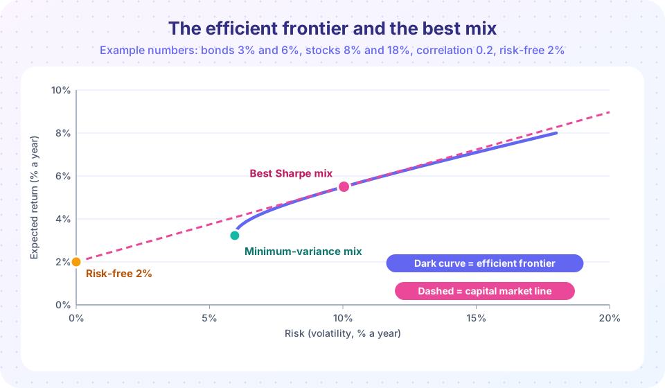
In the last lesson we plotted every stock and bond mix for correlation 0.2. The result is a curve with a leftmost point, the minimum-variance portfolio. From that point up to the stock-only end the curve is the efficient frontier: for any risk level on it, no other mix gives a higher expected return. The lower branch is dominated, so we ignore it.
With more assets the picture becomes a filled area bounded on the left by a curved edge. The edge is the frontier. A computer finds it by solving, for each target return, the problem of minimizing variance. Real use adds constraints: no short selling, a maximum weight per asset, and so on.
Choosing a point on the frontier is a personal decision. A cautious investor picks a point low on the curve, a bolder investor higher up. Nothing in the mathematics says which is better, because that depends on how you feel about risk.
The Sharpe ratio
William Sharpe proposed a way to compare portfolios of different risk:
Sharpe ratio = (expected return - risk-free rate) / volatility
The numerator is the excess return, the reward above what a safe asset pays. The denominator is the risk. So the ratio is "reward per unit of risk". Take our example with a risk-free rate of 2%:
| Portfolio | Return | Volatility | Sharpe ratio |
|---|---|---|---|
| All bonds | 3.0% | 6.0% | 0.17 |
| All stocks | 8.0% | 18.0% | 0.33 |
| 50/50 mix (ρ = 0.2) | 5.5% | 10.0% | 0.35 |
| Minimum variance (4.5% stocks) | 3.2% | 5.95% | 0.21 |
The 50/50 mix has the highest Sharpe ratio of all long-only stock-and-bond mixes in this example, with a Sharpe ratio of about 0.35. This is the tangency portfolio: in the picture, the dashed line from the risk-free point touches the curve exactly there. A steeper line would miss the curve; a flatter one would sit below it. Among all lines from the risk-free point to the frontier, the tangent is the steepest, and its slope is the maximum Sharpe ratio.
Mixing with a risk-free asset
Now suppose you can hold the risk-free asset as well. Mix a fraction x of your money in the tangency portfolio and 1 - x in the risk-free asset. The resulting expected return and volatility are linear in x:
return     = rf + x × (tangency return - rf)
volatility = x × tangency volatility
All such portfolios lie on a straight line, the capital market line. Using our numbers:
- x = 0.5: return 2 + 0.5 × 3.5 = 3.75%, volatility 0.5 × 10.04 = 5.0%.
- x = 1: the tangency portfolio itself, 5.5% return, 10.04% volatility.
- x = 1.5: borrowing half your capital at the risk-free rate to invest more: return 2 + 1.5 × 3.5 = 7.25%, volatility 15.1%.
Every point on this line beats a portfolio on the risky-asset frontier at the same volatility. For instance, at 10% volatility the tangency portfolio is unbeatable, but at 5% volatility, the line offers 3.75% where the curve of risky assets offers less. This leads to the separation theorem: all investors, whatever their risk preference, should hold the same mix of risky assets (the tangency portfolio). They differ only in how much they put into it versus the risk-free asset. A cautious investor holds mostly cash and a bit of the tangency mix; a bold one holds all of it or borrows to hold more. (In reality, borrowing costs more than lending and carries real danger, so treat the right-hand part of the line with caution.)
Using the Sharpe ratio well
The Sharpe ratio is the most popular risk-adjusted performance measure. Use it with care:
- Compare like with like. Use the same period and the same risk-free rate, and annualize consistently. If you compute it from monthly data, multiply the monthly Sharpe by √12.
- It treats upside and downside the same. A fund with large occasional gains looks risky to it. Variants such as the Sortino ratio use only downside volatility.
- Smooth returns can fool it. Funds that report smoothed or infrequently priced values look better than they are.
- It looks backward. A high past Sharpe ratio does not promise a high future one.
A rule of thumb is that a long-run Sharpe ratio of around 0.3 to 0.5 is typical for a broad stock market, but any such number depends on the period and on measurement. A ratio above 1 over a long time is rare, and claims of very high ratios deserve suspicion.
The weakness of optimizers
If the theory is so clean, why doesn't everyone just run an optimizer? Because the output depends heavily on inputs that are hard to know. Expected returns, in particular, are very hard to forecast, and the optimizer treats your estimates as certain. A tiny change in an input can swing the weights wildly; the optimizer tends to pile into the assets whose estimates happen to be too high, an effect called error maximization. The result can be extreme, unstable portfolios.
Practitioners respond in several ways:
- Use constraints, such as no shorting and maximum weights.
- Use shrinkage or Bayesian methods that pull estimates toward sensible defaults.
- Start from a neutral reference, such as the market weights, and adjust only where they have strong views.
- Use simple rules. A well-known study by DeMiguel, Garlappi and Uppal (2009) found that splitting money equally among N assets, the "1/N" rule, was hard to beat out of sample against many sophisticated optimizers, because estimation error swamped the theoretical gain.
The lesson is not that optimization is useless. It is that its value is in the structure, the knowledge that mixes matter, correlations matter and you should not hold dominated portfolios, rather than in false precision.
Common misconceptions
"The highest Sharpe ratio is the right portfolio for everyone." It is the best risky mix, but how much you hold of it relative to cash depends on your risk preference.
"A high Sharpe ratio means a safe fund." It measures return per unit of volatility. A fund can have a high ratio and still lose in a crisis, especially if smoothing hides its true risk.
"The optimizer says to hold 80% in one asset, so I should." Extreme optimizer output is usually a sign of noisy inputs, not insight.
Try it
First, compute the frontier, the tangency mix and the capital market line for the example, then plot it. Change the inputs and see how the best mix moves.
Press Run (or Ctrl + Enter) to see the result here.
Program input · what you'd type while the program runs
Type the answers before you press Run, one per line. Each time the program reads a line (with input()), it gets the next line from this box.
Second, an experiment on fragility: nudge the stock return estimate by one percentage point and see how far the "optimal" weight moves.
Press Run (or Ctrl + Enter) to see the result here.
Program input · what you'd type while the program runs
Type the answers before you press Run, one per line. Each time the program reads a line (with input()), it gets the next line from this box.
Check your understanding
Quick check · 5 questions
of 5 answered You scored / 5 · perfect!
-
1. A portfolio returns 9% with 15% volatility. The risk-free rate is 3%. What is its Sharpe ratio?
(9 - 3) / 15 = 0.40. -
2. Which portfolios lie on the efficient frontier?
Efficient portfolios are not beaten by any alternative with the same or lower risk. -
3. The tangency portfolio is:
It is where the line from the risk-free point just touches the frontier. -
4. According to the separation theorem, how should two investors with different risk preferences differ?
Everyone shares the tangency mix; risk preference sets the split with cash. -
5. Why do optimizers often give unstable weights?
Optimizers take estimates at face value and exploit their errors.
Summary
- The efficient frontier is the set of mixes with the highest expected return for each risk level.
- Sharpe ratio = (return - risk-free rate) / volatility; the tangency portfolio has the highest one.
- Blending the tangency mix with the risk-free asset traces the capital market line; investors differ only in how much they hold of each.
- Optimizers are sensitive to estimated inputs; constraints, shrinkage and simple rules keep them sensible.
Next: CAPM and beta
Track your progress
Create a free account to tick off lessons and pick up where you left off on any device.
of Investing and Markets lessons completed