


















Lesson 14 of 46 · Risk, Return and Diversification
Diversification and correlation: the nearly free lunch
See why mixing assets lowers risk without lowering expected return, how correlation controls the effect, the formula for two assets, and why diversification has limits.
Economist Harry Markowitz is said to have called diversification "the only free lunch in finance". Whether or not he said exactly that, the idea is sound and surprisingly strong. If you mix two investments that do not rise and fall together, the mix is less volatile than the average of its parts, while its expected return is just the average of their returns. You get some risk reduction without paying for it in expected return. This lesson shows why, gives the formula, and explains the conditions under which the lunch gets smaller.
What you will learn
- What correlation is and how to read its values from -1 to +1.
- How to compute the volatility of a two-asset portfolio.
- Why adding more stocks reduces risk, and where the reduction stops.
- When diversification disappoints.
Key terms
Correlation (ρ): a number between -1 and +1 showing how two assets' returns move together.
Covariance: the unscaled measure behind correlation; positive when two returns tend to rise and fall together.
Weight: the share of the portfolio held in an asset.
Diversification benefit: the amount by which portfolio risk is lower than the weighted average of the assets' risks.
Why mixing helps: an intuition
Imagine two businesses on a beach. One sells umbrellas and does well when it rains; the other sells sunscreen and does well when it is sunny. Each business has an uncertain income. Owning both gives you a steadier income than either alone, because bad weather for one is good weather for the other. Their results are negatively related. Even when two assets are only weakly related, one often zigs while the other zags, so the combination fluctuates less than either alone.
Correlation
Correlation captures that relationship in one number, ρ (the Greek letter rho):
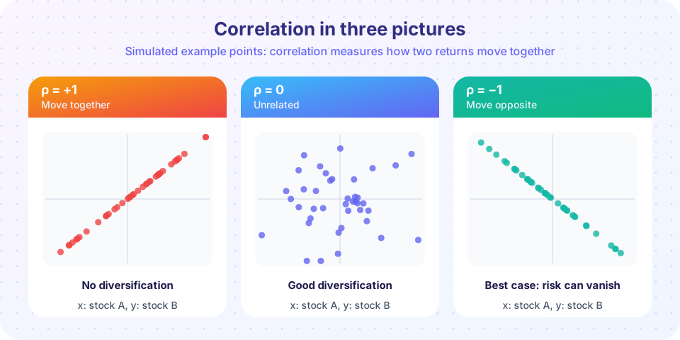
- ρ = +1: perfect positive. The two returns move in the same direction in proportion. No diversification.
- ρ = 0: no linear relationship. The returns wander independently.
- ρ = -1: perfect negative. When one rises, the other falls by a matching amount. A perfect hedge.
The picture shows each case as a cloud of points where one axis is stock A's return and the other is stock B's. Real pairs of assets are in between. Two large US stocks might have a correlation around 0.5 to 0.7. A broad stock index and government bonds have often been near zero or slightly negative over some periods and positive over others. Correlations are not fixed: they change over time, and in a market crash many assets that were weakly related suddenly fall together, so their correlations jump toward +1. That is the main weakness of diversification.
Correlation is computed from the covariance: ρ = covariance(A, B) / (σA × σB). Dividing by the volatilities rescales the result to the range -1 to +1.
The two-asset formula
For a portfolio with weight w in asset A and 1 - w in asset B, the expected return is the weighted average:
E(R) = w × E(A) + (1 - w) × E(B)
The volatility is not the weighted average. It is:
σ = √( w²σA² + (1-w)²σB² + 2 w (1-w) ρ σA σB )
The last term contains ρ. When ρ = 1, the formula collapses to the plain weighted average, σ = wσA + (1-w)σB, so there is no gain. When ρ < 1, the last term is smaller and the portfolio's volatility falls below the average.
A worked example. Two assets each have an expected return of 8% and a volatility of 20%. Put 50% in each. The expected return is 8% whatever the correlation. The volatility depends on ρ, using σ = √(200 × (1 + ρ)) in this symmetric case:
| Correlation | Portfolio volatility |
|---|---|
| +1.0 | 20.0% |
| +0.5 | 17.3% |
| 0 | 14.1% |
| -0.5 | 10.0% |
| -1.0 | 0% |
With ρ = 0 the portfolio is about 30% less volatile and has the same expected return. That is the free lunch: the same expected return for less risk. (It is "nearly" free because it can disappear if correlations rise.)
Many assets: where the benefit stops
With more assets the effect keeps growing but at a decreasing rate. For n equally weighted stocks that each have volatility σ and an average pairwise correlation ρ, portfolio variance is:
σp² = σ² × ( ρ + (1 - ρ) / n )
As n grows, the second term shrinks toward zero and the variance approaches σ²ρ, a floor made of what the stocks have in common. Put numbers in: each stock has σ = 30% and ρ = 0.3.
- 1 stock: 30%
- 10 stocks: about 18.2%
- 30 stocks: about 17.1%
- Many stocks: floor of about 16.4%
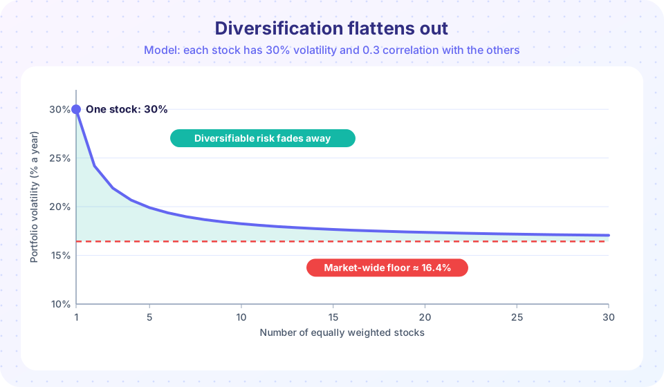
Most of the gain comes from the first 10 to 20 holdings. This floor is market risk, the systematic part from Lesson 3. Everything above the floor is idiosyncratic risk, which diversification removes. That is why a single share can be twice as volatile as the market while paying no more expected return: the market rewards only the floor.
Beyond stocks: diversifying across asset classes, countries and time
Holding 30 stocks from one sector, or one country, leaves you exposed to the shared factors of that sector or country. Real diversification spreads across:
- Asset classes: stocks, bonds, cash, real estate, and others.
- Regions: domestic and international markets, which have different economic cycles.
- Sectors and styles: technology, healthcare, energy, value and growth.
- Time: buying regularly instead of all at once reduces the risk of choosing a bad moment.
A broad index fund does much of this in one purchase, which is why it is the default tool of many long-term investors.
When diversification disappoints
- Crises raise correlation. In 2008 and in 2020, markets worldwide fell together for a time. Diversification helped more over full cycles than in the worst days.
- It cannot create return. It reduces risk for a given expected return; it does not guarantee that you will not lose money.
- Over-diversification. Owning 40 funds that all hold the same stocks adds complexity and cost without adding protection ("di-worsification").
- Hidden concentration. Several funds may all be heavily invested in the same few large companies. Check what you actually own.
Common misconceptions
"A diversified portfolio never loses money." It can fall a lot in a market-wide decline.
"More holdings are always better." Beyond a few dozen stocks the extra benefit is tiny, and costs and overlap can rise.
"Negative correlation is the goal." Even a correlation of zero or a modest positive value gives some benefit. Truly negative pairs are rare and unstable.
Try it
First, compute a correlation from data and the volatility of a 50/50 portfolio. The returns are invented.
Press Run (or Ctrl + Enter) to see the result here.
Program input · what you'd type while the program runs
Type the answers before you press Run, one per line. Each time the program reads a line (with input()), it gets the next line from this box.
Second, the number-of-stocks curve with your own inputs. Change rho to see how the floor moves.
Press Run (or Ctrl + Enter) to see the result here.
Program input · what you'd type while the program runs
Type the answers before you press Run, one per line. Each time the program reads a line (with input()), it gets the next line from this box.
The third block lets you sweep the correlation and watch the 50/50 volatility.
Check your understanding
Quick check · 5 questions
of 5 answered You scored / 5 · perfect!
-
1. Two assets have correlation +1. What is the volatility of a mix?
With perfect positive correlation there is no diversification benefit. -
2. Which correlation gives the biggest risk reduction?
The lower the correlation, the smaller the cross term in the variance formula and the larger the benefit. -
3. Two assets each have 20% volatility and ρ = 0. What is the volatility of a 50/50 mix?
σ = √(200 × (1 + 0)) = √200 ≈ 14.1%. -
4. As you add more and more stocks, portfolio risk approaches a floor. What is that floor made of?
Company-specific risk averages out; what the stocks have in common remains. -
5. Why can diversification disappoint during a crisis?
In a panic many assets sell off together, reducing the usual benefit.
Summary
- Correlation ranges from -1 to +1; the lower it is, the more mixing assets reduces volatility.
- Two-asset volatility: σ = √(w²σA² + (1-w)²σB² + 2w(1-w)ρσAσB); expected return is the plain weighted average.
- Many-stock volatility approaches a floor √ρ × σ: market risk remains, company risk disappears.
- Diversify across asset classes, regions and time; beware crisis-time correlations and hidden overlap.
Next: Chapter 3 review
Track your progress
Create a free account to tick off lessons and pick up where you left off on any device.
of Investing and Markets lessons completed