


















Lesson 25 of 46 · Stocks and Valuation
Dividend Discount and DCF Valuation
Value a stock from its future cash: the Gordon growth formula, discounted cash flow, terminal value, net debt and a sensitivity table, with runnable examples.
Multiples compare a company with others. Discounted cash flow valuation compares it with itself: it asks what the cash the business will produce in the future is worth today. The core idea is the time value of money. A dollar you receive in five years is worth less than a dollar today, because today's dollar could be invested and grow. If you demand a return of r per year, then a payment of C in t years is worth C / (1 + r)^t now. That division is called discounting, and r is the discount rate.
This lesson builds two models on that idea. The dividend discount model is the simplest and works for steady dividend payers. The free cash flow model is the workhorse for everything else.
What you will learn
- How to value a growing dividend stream with the Gordon growth formula.
- How to forecast free cash flow, discount it, and add a terminal value.
- How to move from enterprise value to a value per share using net debt.
- How to read a sensitivity table and a reverse DCF to see what the market price implies.
Key terms
Present value: today's worth of a future payment, found by discounting.
Terminal value: the value at the end of the forecast of all cash flows after it.
Net debt: debt minus cash.
WACC: the weighted average cost of capital, the discount rate for the cash flows of the whole business.
Reverse DCF: solving for the growth that makes the model's value equal the market price.
The Gordon growth model
If a company pays a dividend this year of D0 and you expect it to grow forever at a steady rate g, then next year's dividend is D1 = D0 x (1 + g). Summing the discounted dividends forever collapses, by the formula for a geometric series, into one line:
P = D1 / (r - g)
This is the Gordon growth model, named after Myron Gordon. It requires r > g; otherwise the sum does not converge and the formula gives nonsense. In practice g must also be at most the long-run growth rate of the economy, since no company can outgrow it forever.
Example with an invented electricity utility, Northgate Power. It paid 2.00 per share this year, you expect 3 percent yearly growth, and given its risk you require 8 percent. Then D1 = 2.06 and P = 2.06 / (0.08 - 0.03) = 41.20. Raise the required return to 9 percent and the value drops to 2.06 / 0.06 = 34.33; cut it to 7 percent and it rises to 51.50. A one-point change in the discount rate moves the value by 20 to 25 percent, a first warning about how sensitive these models are.
The model suits companies with stable, mature dividends such as regulated utilities. It fails for companies that pay no dividend, which includes many of the largest ones, and it ignores that a company's payout can change. For those, value the cash the business generates rather than the cash it chooses to pay out.
Free cash flow valuation
The free cash flow model works in five steps.
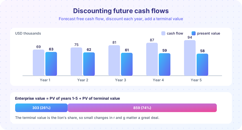
1. Forecast free cash flow. You met free cash flow in the statements lesson: operating cash flow less capital spending. Brightwater's last year was 64. Suppose you expect it to grow 8 percent a year for five years: 69.1, 74.6, 80.6, 87.1, 94.0.
2. Choose the discount rate. For cash flows that belong to all the providers of capital, use the WACC: the cost of equity and the after-tax cost of debt, weighted by how the company is financed. The cost of equity is often estimated with the capital asset pricing model, r = risk-free rate + beta x equity risk premium; for example 4% + 1.1 x 5% = 9.5%. Our simplified example uses a 10 percent WACC.
3. Discount each year. Year 1's 69.1 divided by 1.10 is 62.8; year 5's 94.0 divided by 1.10^5 is 58.4. Together the five years are worth 303.
4. Add a terminal value. The business does not end in year 5. Assume that after year 5 cash flow grows at a modest 3 percent forever. The Gordon formula, applied to cash flow, gives the value at the end of year 5: TV = FCF5 x (1 + g) / (WACC - g) = 94.0 x 1.03 / 0.07, about 1,384. Discounted back five years, it is worth about 859 today.
5. Add and adjust. The sum, 303 + 859 = 1,162, is the enterprise value: what the whole operating business is worth. Shareholders own what is left after the lenders are paid, so subtract net debt (debt 390 minus cash 150, or 240): equity value is 922. Divide by 100 thousand shares and the model gives about 9.22 per share.
The market price of 18.00 is nearly twice that. Does that make the stock a sell? Not by itself. The model is only as good as its inputs, and it is telling you something about expectations, which the next section explores.
Where the value sits
Notice that the terminal value is roughly 74 percent of the enterprise value, even though it is a single number far in the future. This is typical. It means the long-run growth rate and the discount rate matter more than the details of the next five years. The sensitivity heat map in the third example below makes this visible: vary the discount rate by 1 point and the terminal growth by 1 point and the value per share swings widely.
Good practice follows from this. Keep terminal growth modest (at or below long-run inflation plus a little real growth), forecast long enough that the business reaches a steady state before the terminal year, and show a table of values for different assumptions rather than a single figure.
Reverse DCF: what is the market assuming?
Instead of asking "what is it worth?", ask "what must be true for the price to be right?" Fix the discount rate and terminal growth, then solve for the five-year growth rate that produces a value of 18.00 per share. If the answer is 20 percent a year for five years, you can ask whether that is plausible for a coffee roaster. A reverse DCF turns an argument about numbers into an argument about assumptions, which is more productive. The second example below does the solving by trial and error and finds that the price of 18.00 needs growth of about 22 percent a year for five years, far above the 8 percent we assumed.
Common misconceptions
"The DCF gives the true value." It gives the value implied by your assumptions. Different, equally reasonable assumptions give a wide range.
"A higher growth rate is always better." Growth that requires heavy investment does not help unless the return on that investment exceeds the discount rate.
"Terminal value is a technicality." It is usually the largest part of the value; scrutinize it first.
"Debt is irrelevant after computing enterprise value." Enterprise value belongs to lenders and owners together; subtract net debt to get the owners' share.
Try it
First, the Gordon model with a grid of discount rates and growth rates. Notice how the value explodes when r - g becomes small.
Press Run (or Ctrl + Enter) to see the result here.
Program input · what you'd type while the program runs
Type the answers before you press Run, one per line. Each time the program reads a line (with input()), it gets the next line from this box.
Second, a full free cash flow valuation with a table of each year, a per-share result, and a reverse DCF that finds the growth rate hidden in a given price.
Press Run (or Ctrl + Enter) to see the result here.
Program input · what you'd type while the program runs
Type the answers before you press Run, one per line. Each time the program reads a line (with input()), it gets the next line from this box.
Third, a sensitivity heat map for value per share over a range of discount rates and terminal growth rates.
Press Run (or Ctrl + Enter) to see the result here.
Program input · what you'd type while the program runs
Type the answers before you press Run, one per line. Each time the program reads a line (with input()), it gets the next line from this box.
Check your understanding
Quick check · 5 questions
of 5 answered You scored / 5 · perfect!
-
1. A stock pays 1.50 this year, dividends are expected to grow 4% a year forever, and you require 9%. What does the Gordon model give?
D1 = 1.50 x 1.04 = 1.56, and 1.56 / (0.09 - 0.04) = 31.20. -
2. What must hold for the Gordon growth formula to work?
If growth were at least equal to the discount rate, the present values would never shrink and the sum would not converge. -
3. In the free cash flow model, what does subtracting net debt do?
Lenders have the first claim on the enterprise value; what remains belongs to shareholders. -
4. Why is the terminal value so important in a typical DCF?
A single number representing all cash flows beyond the forecast period usually dominates, so g and the discount rate matter a lot. -
5. What does a reverse DCF tell you?
It solves for the assumption that makes the model equal the price, so you can judge whether it is plausible.
Summary
- Discounting converts future cash to present value:
C / (1 + r)^t. - The Gordon model,
P = D1 / (r - g), values a steadily growing dividend and needsr > g. - A free cash flow DCF adds forecast cash flows and a terminal value, giving enterprise value; subtract net debt for equity value.
- Terminal value dominates, so test the discount rate and terminal growth with a sensitivity table or reverse DCF.
- A DCF value is an estimate that depends on assumptions, not a fact.
Next: Chapter review
Track your progress
Create a free account to tick off lessons and pick up where you left off on any device.
of Investing and Markets lessons completed