


















Lesson 38 of 45 · Working Capital and Valuation
Valuation multiples and sensitivity analysis
Value a company with EV/EBITDA and P/E multiples from comparable firms, understand what drives a multiple, and stress-test any valuation with sensitivity grids and scenarios.
A DCF starts from first principles and takes a lot of work. Most day-to-day valuation instead starts from a shortcut: what are similar businesses worth? If four comparable companies trade at about seven times their operating cash earnings, a fifth probably will too. This is relative valuation, and it is how brokers, bankers and buyers quickly size up a price. It is also easy to misuse, so this lesson covers both the craft and the cautions. We finish with sensitivity analysis, the habit that turns any single-number valuation into an honest range.
What you will learn
- Compute common equity and enterprise multiples and apply them to a target company.
- Pair numerators and denominators consistently.
- Choose comparables and explain what drives a multiple.
- Build one-way and two-way sensitivity tables and scenario-weighted values.
- Summarize a valuation as a range.
Key terms
Multiple: value divided by a financial measure, such as EV/EBITDA. EBITDA: earnings before interest, taxes, depreciation and amortization. P/E: share price divided by earnings per share. Comparable (peer): a similar listed company used as a benchmark. Sensitivity analysis: re-computing value as one or two inputs change.
Common multiples
Enterprise multiples compare enterprise value (the whole operating business) with a measure available to all investors: EV/EBITDA, EV/EBIT and EV/Sales. They ignore capital structure, so they suit comparing firms with different debt levels. EBITDA multiples are especially popular for capital-intensive firms, though remember EBITDA ignores the capital spending a firm needs to keep earning it.
Equity multiples compare share price or equity value with a measure that belongs to shareholders: P/E (price over earnings per share), P/B (price over book value per share) and P/S. They are affected by leverage because earnings are after interest.
The rule that avoids nonsense: match the numerator and denominator. Enterprise value, which includes debt, belongs with a pre-interest measure (EBITDA, EBIT, sales). Price or equity value belongs with a post-interest measure (net income, book equity). Dividing EV by net income mixes claims and gives a meaningless number.
A worked example
Northwind Cycles (the company from the DCF lesson) has EBITDA of $200 million, net debt of $300 million, 100 million shares and net income of $76.5 million (EBIT 120, interest 18, tax 25%: (120 − 18) × 0.75 = 76.5). Five peers, invented for illustration, trade at these EV/EBITDA multiples: 6.5, 7.0, 7.4, 8.0, 8.1. The median is 7.4. (Medians resist the pull of outliers.)
- Implied EV =
200 × 7.4 = $1,480 million. - Implied equity =
1,480 − 300 = $1,180 million, or $11.80 per share.
For P/E: Northwind's EPS is 76.5 / 100 = $0.765. If peers have a median P/E of 14, the implied price is 0.765 × 14 ≈ $10.71.
Compare with the DCF value of $11.48 per share: the three methods bracket roughly $10.7 to $11.8. That agreement is reassuring, not proof. A wide gap would be a prompt to examine whether the DCF forecast, the peer group or the multiple's assumptions are off.
Press Run (or Ctrl + Enter) to see the result here.
Program input · what you'd type while the program runs
Type the answers before you press Run, one per line. Each time the program reads a line (with input()), it gets the next line from this box.
What drives a multiple
A multiple is a compressed DCF. For a steady-growth firm, EV/EBITDA is higher when growth is higher, when reinvestment needs are lower (so more EBITDA turns into free cash flow) and when the discount rate is lower. A "justified" P/E for a growing dividend payer is
P/E = payout ratio × (1 + g) / (Re − g)
with a similar structure to the Gordon formula. This explains patterns: high-growth firms trade at high multiples; risky firms at low ones; capital-heavy firms at lower EBITDA multiples than asset-light ones, because more of their EBITDA is consumed by capital spending.
Choosing comparables is therefore about matching these drivers: same industry, similar growth and margins, similar risk and size, same region or accounting rules. Adjust for one-off items, and compare like with like (trailing earnings with trailing, forward with forward).
Cautions
- The peers can be wrong together. If the whole sector is over-excited, a multiple valuation inherits the bubble. A DCF can at least show what growth the market is assuming.
- Accounting differences. Leases, depreciation methods and one-offs distort earnings across firms and countries.
- Negative or tiny earnings make P/E meaningless; use sales or EBITDA multiples.
- Single-number comfort. A multiple hides every assumption inside it.
Sensitivity analysis: how wrong could we be?
Every valuation rests on uncertain inputs. Sensitivity analysis re-computes value as inputs change.
- One-way: vary a single input (say WACC from 8% to 10%) and watch the result.
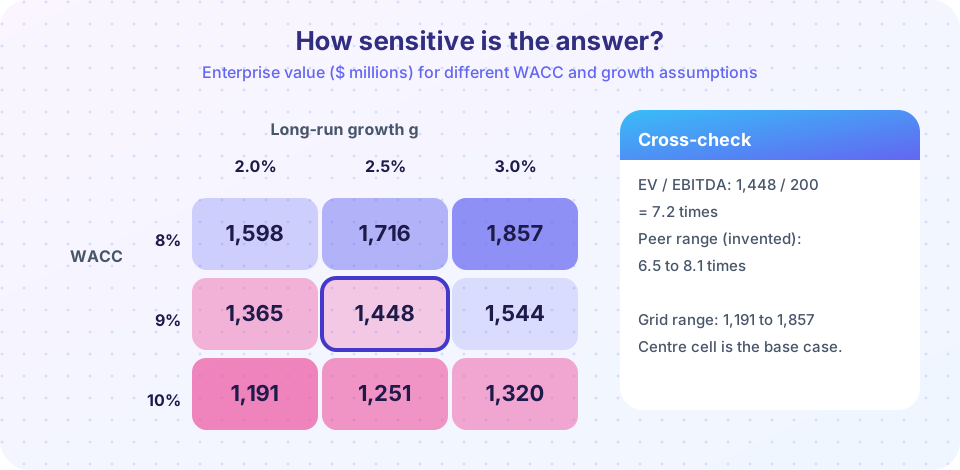
- Two-way grid: vary two inputs at once. The grid in the picture shows enterprise value for WACC 8-10% and growth 2-3%: the centre (1,448) is the base case, but the range from 1,191 to 1,857 spans a spread of nearly half the base value, from only modest changes to two inputs.
- Scenarios: define coherent bear, base and bull cases, where several inputs move together (weaker sales, higher discount rate), and weight them by probability.
- Tornado chart: rank inputs by the swing they cause, so you know where research effort is worth spending.
- Monte Carlo simulation: draw inputs from distributions many times and look at the spread of values.
The goal is not an impressive spreadsheet but a decision-relevant statement: "Under reasonable assumptions the company is worth $10 to $13 per share; the market price of $9 sits below the range." A football-field chart, which stacks the ranges from DCF, multiples and other methods, is the standard way to present this to a board.
Press Run (or Ctrl + Enter) to see the result here.
Program input · what you'd type while the program runs
Type the answers before you press Run, one per line. Each time the program reads a line (with input()), it gets the next line from this box.
Common misconceptions
"A cheap multiple means a cheap company." A low multiple may reflect low growth, high risk or poor capital efficiency. Cheap and good value are different things.
"Multiples are objective and DCF is subjective." Both rely on judgments: multiples hide them in the choice of peers, period and adjustments.
"One sensitivity table covers all the risk." A grid varies only the inputs you chose. Structural risks (a lost customer, a new competitor) need scenarios.
Check your understanding
Quick check · 5 questions
of 5 answered You scored / 5 · perfect!
-
1. A company has EBITDA of $50m and net debt of $80m. Peers trade at a median 9x EV/EBITDA. What is the implied equity value?
EV = 50 × 9 = 450; equity = 450 − 80 = $370m. -
2. Which pairing of numerator and denominator is consistent?
EV includes debt, so pair it with a pre-interest measure such as EBITDA. -
3. EPS = $2.00 and the peer median P/E is 15. What is the implied price?
Price = EPS × P/E = 2.00 × 15 = $30.00. -
4. Why is the median often preferred to the mean for peer multiples?
One extreme peer can distort an average but barely moves a median. -
5. What is a two-way sensitivity table?
It shows value across a grid of values of two assumptions, such as WACC and growth.
Summary
- Multiples price a firm relative to peers; match enterprise value with pre-interest measures and equity value with post-interest ones.
- A multiple compresses growth, risk and reinvestment; pick peers that match those drivers.
- Sensitivity grids, scenarios and simulation turn a point estimate into a range; present the range.
Next: Chapter review
Track your progress
Create a free account to tick off lessons and pick up where you left off on any device.
of Corporate Finance lessons completed