


















Lesson 32 of 45 · Capital Structure and Payout
The trade-off theory and the debt decision
See how the tax shield, financial distress costs and agency costs combine into a target debt ratio, compare it with the pecking order view, and test leverage with EBIT-EPS analysis.
Modigliani and Miller's tax result says "borrow more, forever". Reality says otherwise: airlines, steelmakers and plenty of well-run firms keep debt moderate, and lenders themselves cap how much they will lend. Something offsets the tax shield. This lesson names that something, shows how the two forces combine into a target debt ratio and then asks a practical question every manager faces: if we need $100 million, should we sell shares or borrow?
What you will learn
- Define direct and indirect costs of financial distress.
- Write the static trade-off formula and find the optimum in a numeric model.
- Describe agency costs of debt and equity and the pecking order theory.
- Explain why capital structures differ across industries.
- Compare two financing plans with EBIT-EPS analysis and find the break-even EBIT.
Key terms
Financial distress: trouble meeting obligations to lenders. Agency cost: value lost because managers, shareholders and lenders have conflicting interests. Debt overhang: reluctance to fund good projects because the gains go to lenders. Pecking order: a preference for internal funds, then debt, then equity. Financial leverage: use of fixed financing costs that magnify the effect of earnings on shareholders.
Costs of financial distress
A firm with a lot of debt has big fixed payments. If profits dip, it may be unable to pay. The consequences are costly in two ways.
Direct costs arise in bankruptcy proceedings: legal and administrative fees, court time and the managers' attention. Studies estimate them at a modest slice of firm value, often a few percent, though they can be larger for smaller firms.
Indirect costs are usually bigger and begin before any filing. Customers worry about warranties and stop buying a product from a shaky seller. Suppliers demand cash on delivery. Good employees leave. Managers cancel profitable long-term projects to save cash. Assets are sold quickly at fire-sale prices. These costs depend on how specific the firm's assets are: a company holding standard, resaleable property (a landlord) loses little in distress; a company whose value lies in brand, software or human skill loses a lot.
The expected cost is probability of distress × cost if it happens. Both rise with debt, so the expected distress cost climbs ever more steeply as leverage increases.
The static trade-off model
Putting the tax benefit of debt beside the cost gives
V_L = V_U + PV(interest tax shield) − PV(expected distress costs)
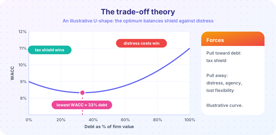
Because the shield grows roughly in a straight line (T × D) while distress costs accelerate, value rises with debt at first, peaks, then falls. At the peak, the marginal benefit of another dollar of debt equals the marginal cost. Because WACC mirrors value (a higher firm value corresponds to a lower WACC for the same cash flows), the same logic yields the U-shaped WACC curve above.
Here is a small numeric model. Take V_U = 750, T = 25%, an expected distress cost that grows as 0.30 × V_U × (D/800)³ (capped at the full cost), and search for the best debt level. The code below prints it.
Press Run (or Ctrl + Enter) to see the result here.
Program input · what you'd type while the program runs
Type the answers before you press Run, one per line. Each time the program reads a line (with input()), it gets the next line from this box.
With these invented parameters the best debt level comes out at about $436 million, roughly 53% of firm value. A different distress-cost shape moves the peak (the curve in the picture peaks near 33%), which is exactly the point: the structure of the argument is solid, but the optimum is only as good as the guesses behind it.
Agency costs
Conflicts of interest add more forces:
- Asset substitution (risk shifting). When a firm is near distress, shareholders have an incentive to take big gambles: if they win, shareholders keep the upside; if they lose, lenders absorb the loss. Lenders anticipate this and charge more or add restrictive covenants.
- Debt overhang. A heavily indebted firm may skip a profitable project because most of its payoff would go to lenders, not shareholders. Value that should have been created is lost.
- Discipline benefit. Michael Jensen argued that fixed debt payments force managers to pay out spare cash instead of wasting it on empire-building. This is a pro-debt agency effect, strongest for mature firms generating lots of free cash with few good projects.
The pecking order and signalling
Stewart Myers and Nicholas Majluf proposed a different story. Managers know more about the firm than outsiders do. If they issue shares, outsiders suspect they think the stock is overpriced, and the share price drops. So firms prefer funding projects with retained earnings, then debt, and only as a last resort new equity. Under this view there is no target ratio; the debt ratio is simply the accumulated result of past financing needs. Evidence shows both forces at work: firms do appear to move toward targets slowly, and announcements of equity issues are, on average, met with price falls.
Patterns across industries
A rough but useful regularity: firms with stable cash flows and tangible, resaleable assets (utilities, real estate, shipping) can carry more debt; firms whose value lies in intangibles and growth options (software, biotech) tend to use little. Profitable firms sometimes use less debt than expected, which fits the pecking order (they can fund themselves). Treat all of these as tendencies, not rules.
Leverage and earnings: EBIT-EPS analysis
Managers often compare financing plans by looking at earnings per share. Suppose a firm with 10 million shares needs $100 million. It can (A) sell 4 million new shares at $25 each, or (B) borrow $100 million at 8%, costing $8 million of interest. The tax rate is 25%.
- Plan A (equity): 14 million shares, no interest.
EPS = EBIT × 0.75 / 14. - Plan B (debt): 10 million shares.
EPS = (EBIT − 8) × 0.75 / 10.
At the break-even EBIT the two give the same EPS:
EBIT / 14 = (EBIT − 8) / 10 → 10 × EBIT = 14 × EBIT − 112 → EBIT = 28
Above $28 million of operating profit, the debt plan gives higher EPS; below it, the equity plan does. That is financial leverage at work: debt amplifies EPS in good years and cuts it in bad. The degree of financial leverage, DFL = EBIT / (EBIT − Interest), measures the amplification: at EBIT of $40 million, DFL = 40/32 = 1.25, so a 10% change in EBIT moves EPS by about 12.5%.
Press Run (or Ctrl + Enter) to see the result here.
Program input · what you'd type while the program runs
Type the answers before you press Run, one per line. Each time the program reads a line (with input()), it gets the next line from this box.
But beware: a higher EPS under debt is not a higher value. Debt makes EPS riskier, and, by Modigliani-Miller, the extra expected EPS is compensation for that extra risk. EBIT-EPS analysis shows what happens to earnings; the trade-off theory tells you whether value moves.
Common misconceptions
"The optimal debt ratio is a precise number you can compute." Models give a region, not a point. The inputs (distress probabilities and costs) are very hard to estimate, so practitioners pick a target range and a credit rating they want to keep.
"Higher EPS from borrowing means shareholders are better off." Only if the extra EPS exceeds compensation for extra risk. Look at value, not EPS.
"A firm should borrow to the maximum because of the tax shield." The shield is real but is offset by distress and agency costs, and it only helps while the firm earns enough taxable profit to use it.
Check your understanding
Quick check · 6 questions
of 6 answered You scored / 6 · perfect!
-
1. In the static trade-off theory, firm value is maximized where:
Beyond that point extra debt costs more in expected distress than it saves in tax. -
2. Which is an INDIRECT cost of financial distress?
Lost sales, supplier terms and departing staff arise before bankruptcy and can be larger than legal fees. -
3. According to the pecking order theory, what is the first choice for funding?
Internal funds avoid the signalling and issue costs of outside funding. -
4. Plan A: 14m shares, no interest. Plan B: 10m shares, $8m interest. T does not matter for the break-even. What is the break-even EBIT?
EBIT/14 = (EBIT − 8)/10 gives EBIT = 28. -
5. EBIT = $50m and interest = $10m. What is the degree of financial leverage?
DFL = EBIT / (EBIT − interest) = 50 / 40 = 1.25. -
6. Which firm would you expect to use the most debt?
Stable cash flows and resaleable assets lower both the chance and the cost of distress.
Summary
V_L = V_U + PV(tax shield) − PV(distress costs); the optimum balances them.- Distress costs include indirect effects like lost customers and cancelled projects.
- Agency conflicts and information asymmetry (the pecking order) add further forces.
- EBIT-EPS analysis finds the break-even EBIT, but EPS is not value.
Next: Dividends and buybacks
Track your progress
Create a free account to tick off lessons and pick up where you left off on any device.
of Corporate Finance lessons completed