


















Lesson 22 of 45 · Risk and Return
Return and variance: measuring risk
Compute holding-period returns, expected return, variance and standard deviation, compare arithmetic and geometric averages, and understand the risk premium.
You cannot manage what you cannot measure, and risk feels too slippery to measure. Yet finance has a plain answer: describe the spread of the returns you might earn. A savings account that always pays 3% has no spread. A share that might return -30% or +50% has a wide one. In this lesson you will learn the standard measures, work them out by hand on a small example, and learn the traps that catch beginners.
What you will learn
- Compute a holding-period return, including dividends.
- Find an expected return and a variance from a table of scenarios.
- Explain what a standard deviation tells you and what it does not.
- Tell the arithmetic average from the geometric average and know when to use each.
- Define the risk premium and the role of the risk-free rate.
Key terms
Holding-period return: total gain over the period divided by the starting value. Expected return: probability-weighted average of possible returns. Variance: probability-weighted average of squared deviations from the expected return. Standard deviation: square root of the variance, in the same units as returns. Risk premium: expected return minus the risk-free return.
Returns: the raw material
Suppose you buy a share for $50. During the year it pays a dividend of $1.50 and ends at $54. Your gain is the $4 price rise plus the $1.50 dividend, so the holding-period return is
R = (P1 − P0 + D) / P0 = (54 − 50 + 1.5) / 50 = 0.11 = 11%
Always include income as well as price change; ignoring dividends understates the return of an income-paying asset. Returns are fractions of the starting amount, which makes a $50 share and a $5,000 fund comparable.
Returns are also forward-looking when we discuss risk. Before the year starts you do not know R. You can only list what might happen and how likely each outcome is. That list, called a probability distribution, is the starting point for everything that follows.
Expected return from scenarios
Take an invented company, Harbor Foods, and three states of the economy:
| State | Probability | Return |
|---|---|---|
| Recession | 25% | -12% |
| Normal | 50% | +9% |
| Boom | 25% | +26% |
The expected return is the probability-weighted average:
E(R) = 0.25 × (−12) + 0.50 × 9 + 0.25 × 26 = −3 + 4.5 + 6.5 = 8%
Notice that 8% is not one of the outcomes. It is a long-run balance point, not a promise. In a given year you will earn -12%, 9% or 26%.
Variance and standard deviation
To measure the spread, take each outcome's distance from the expected return, square it so that gains and losses do not cancel, and average with the probabilities as weights:
σ² = Σ p × (R − E(R))²
For Harbor Foods the deviations are -20, +1 and +18 percentage points:
σ² = 0.25 × 400 + 0.50 × 1 + 0.25 × 324 = 100 + 0.5 + 81 = 181.5
The unit of variance is "percent squared", which is hard to picture. Taking the square root brings us back to percent:
σ = √181.5 ≈ 13.5%
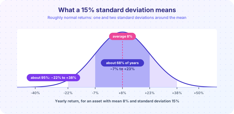
Read this as "a typical year lands roughly 13 to 14 points away from the average". If returns are roughly bell-shaped, about two-thirds of years fall within one standard deviation of the mean, and about 95% within two. For an asset with mean 8% and σ = 15%, that is the band from -7% to 23% in one-sigma terms, and -22% to 38% in two-sigma terms, as in the picture above.
Press Run (or Ctrl + Enter) to see the result here.
Program input · what you'd type while the program runs
Type the answers before you press Run, one per line. Each time the program reads a line (with input()), it gets the next line from this box.
Estimating from history
In practice we rarely know probabilities; we have a record of past returns. With n yearly returns, estimate the mean as the simple average and the variance with a divisor of n − 1 (the sample variance, which corrects for estimating the mean from the same data). Long histories of large listed shares in major markets show average returns several points above short-term government bills, together with yearly standard deviations in the high teens of percent. The exact figures depend on country and period, which is a warning in itself: past statistics are estimates with their own error, not constants of nature.
Arithmetic versus geometric average
Say an investment returns +20%, -10% and +15% in three years. The arithmetic average is (20 − 10 + 15)/3 = 8.33%. But $100 grows to 100 × 1.20 × 0.90 × 1.15 = $124.20, which is a compound annual rate of
(1.2 × 0.9 × 1.15)^(1/3) − 1 ≈ 7.5%
That is the geometric average, the rate that actually compounds your money. The geometric average is always at or below the arithmetic average, and the gap widens as returns become more volatile. A rough rule is geometric ≈ arithmetic − σ²/2. Use the arithmetic average as the best estimate of a typical single year's expected return (it is what goes into forecasts and the CAPM), and the geometric average to describe realized growth over many years.
Press Run (or Ctrl + Enter) to see the result here.
Program input · what you'd type while the program runs
Type the answers before you press Run, one per line. Each time the program reads a line (with input()), it gets the next line from this box.
The risk premium
The least risky asset available, such as a short-term government bill in a stable economy, earns the risk-free rate, rf. Any risky asset's risk premium is its expected return minus rf. If Harbor Foods has E(R) = 8% and bills pay 3%, the premium is 5 percentage points. The premium is the price of bearing Harbor's risk. The next two lessons ask how big it should be, and why only part of Harbor's risk deserves a premium at all.
Common misconceptions
"Standard deviation is the chance I lose money." No. It measures spread in both directions. An asset with a large standard deviation can still have a low chance of loss if its mean is high.
"The arithmetic average is what I earned." Only the geometric average tells you the compound rate you actually earned. Averaging percentages overstates growth when returns are volatile.
"A history of high returns means high future returns." Estimated averages are noisy. A few decades of data leave wide uncertainty about the true mean.
Try it
Two short experiments. The first (above) shows volatility drag. The next is an interactive explorer: change the mean and standard deviation and watch the 68% and 95% bands move.
Check your understanding
Quick check · 5 questions
of 5 answered You scored / 5 · perfect!
-
1. A share bought at $40 pays $2 in dividends and is worth $42 a year later. What is the holding-period return?
(42 − 40 + 2) / 40 = 4 / 40 = 10%. -
2. Scenarios: 50% chance of +10% and 50% chance of −2%. What is the expected return?
0.5 × 10 + 0.5 × (−2) = 5 − 1 = 4%. -
3. For the same scenarios, what is the standard deviation?
Each outcome is 6 points from the mean 4%, so variance = 36 and σ = 6. -
4. Returns of +50% and −50% in two years give an arithmetic average of 0%. What happens to $100?
100 × 1.5 × 0.5 = 75. The geometric average is negative even though the arithmetic average is zero. -
5. Which average should you use as the expected return for ONE future year?
The arithmetic average is the unbiased estimate of a single year's expected return; the geometric average describes compound growth over many years.
Summary
- Return = (price change + income) / starting value.
- Expected return weights outcomes by probability; variance weights squared deviations.
- Standard deviation brings the spread back to percent and is the standard risk measure.
- The geometric average is below the arithmetic average, and volatility widens the gap.
- Risk premium = expected return − risk-free rate.
Next: Diversification
Track your progress
Create a free account to tick off lessons and pick up where you left off on any device.
of Corporate Finance lessons completed