


















Lesson 23 of 45 · Risk and Return
Diversification and portfolio risk
See why combining assets lowers risk, how correlation controls the benefit, and why diversification stops at market risk. Includes worked examples and simulations.
"Don't put all your eggs in one basket" is one of the oldest pieces of advice in money. Finance turns it into arithmetic. A portfolio's expected return is just the weighted average of its parts, but its risk is usually less than the weighted average of the parts' risks. That gap is a free lunch, and it is the only free lunch finance offers. This lesson shows where it comes from, how big it can be, and why it has a floor.
What you will learn
- Compute the expected return and standard deviation of a two-asset portfolio.
- Explain how correlation decides how much risk diversification removes.
- Show why risk falls as the number of assets grows, but never to zero.
- Distinguish unique (diversifiable) risk from market (systematic) risk.
- Find the minimum-variance mix of two assets.
Key terms
Portfolio: a collection of assets held together, described by weights that add to 1. Covariance: how two returns move together. Correlation (ρ): covariance scaled to lie between −1 and +1. Unique risk: risk specific to one company. Market (systematic) risk: risk shared by almost all assets.
Return is easy; risk is subtle
Consider two invented assets. Asset A has expected return 10% and standard deviation 20%. Asset B has expected return 6% and standard deviation 12%. Put half your money in each.
The expected return is a plain weighted average:
E(Rp) = 0.5 × 10 + 0.5 × 6 = 8%
Risk is not. The portfolio variance of two assets is
σp² = wA²σA² + wB²σB² + 2 wA wB ρ σA σB
where ρ is the correlation between the two returns. Plugging in the numbers with ρ = 0.3:
σp² = 0.25×0.04 + 0.25×0.0144 + 2×0.25×0.3×0.2×0.12 = 0.01 + 0.0036 + 0.0036 = 0.0172
so σp = √0.0172 ≈ 13.1%. The average of the two standard deviations is 16%, yet the portfolio's risk is only 13.1%. The two assets do not move in lockstep, so a bad year for one is partly cushioned by the other.
Correlation is the dial
The cross term is the whole story. Keep the same weights and vary ρ:
| Correlation ρ | Portfolio σ | Comment |
|---|---|---|
| +1.0 | 16.0% | no benefit: the plain average |
| +0.3 | 13.1% | modest benefit |
| 0.0 | 11.7% | independent assets |
| −0.5 | 8.7% | strong benefit |
| −1.0 | 4.0% | risk can almost vanish |
At ρ = +1 diversification does nothing. At any ρ below +1 it helps, and the lower the correlation, the bigger the help. Real assets rarely have correlations near −1; two shares in the same industry might sit at +0.7, shares in different industries at +0.3 to +0.5, and bonds against stocks anywhere from slightly negative to moderately positive depending on the period. Seeking low-correlation assets is the practical craft of diversification.
Press Run (or Ctrl + Enter) to see the result here.
Program input · what you'd type while the program runs
Type the answers before you press Run, one per line. Each time the program reads a line (with input()), it gets the next line from this box.
The shape of the opportunity set
Vary the weight in A from 0 to 1 and plot risk against return. For ρ = 1 you get a straight line between the two assets. For lower ρ the line bows to the left: you can reach the same return with less risk. For ρ = 0.3 the leftmost point is the minimum-variance portfolio. Setting the derivative of the variance to zero gives its weight in A:
wA = (σB² − ρσAσB) / (σA² + σB² − 2ρσAσB) = (0.0144 − 0.0072) / 0.0400 = 0.18
Only 18% in the riskier asset gives the lowest possible risk. Remarkably, that mix is less risky than holding B alone, even though B is the safer asset. Portfolios on the upper half of the bow are efficient: no other mix offers more return for the same risk. Choosing among them depends on how much risk you can tolerate.
Press Run (or Ctrl + Enter) to see the result here.
Program input · what you'd type while the program runs
Type the answers before you press Run, one per line. Each time the program reads a line (with input()), it gets the next line from this box.
Many assets: why risk falls, and where it stops
With n equally weighted assets, each with variance σ² and every pair having covariance C, the portfolio variance is
σp² = σ²/n + (1 − 1/n) × C
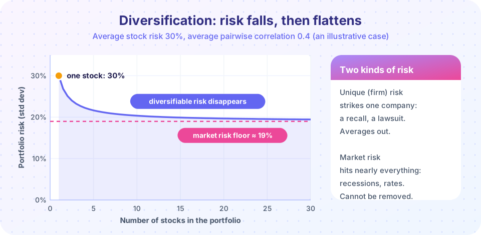
The first term, the average of the individual variances divided by n, vanishes as n grows. The second term approaches the average covariance and does not. So portfolio risk falls toward √C.
Take an illustrative set of stocks each with σ = 30% (variance 0.09) and an average pairwise correlation of 0.4, so C = 0.4 × 0.09 = 0.036:
- n = 1: σp = 30.0%
- n = 10: σp = √(0.036 + 0.054/10) ≈ 20.3%
- n = 30: σp ≈ 19.4%
- n → ∞: σp → √0.036 ≈ 19.0%
Two lessons. First, most of the benefit arrives with the first ten to twenty holdings. Second, the floor of about 19% is not zero. What remains is market risk (also called systematic or non-diversifiable risk): recessions, interest-rate moves, and anything else that pushes many companies in the same direction at once. The part that disappears is unique risk (also called idiosyncratic or diversifiable): a factory fire, a lost lawsuit, a failed product.
Press Run (or Ctrl + Enter) to see the result here.
Program input · what you'd type while the program runs
Type the answers before you press Run, one per line. Each time the program reads a line (with input()), it gets the next line from this box.
Why the market pays only for market risk
Suppose investors were paid a premium for unique risk. Then a clever investor could buy many such assets, wipe out the unique risk by diversifying, and keep the premium: a free profit. Demand would raise those prices and push expected returns down until the premium vanished. Therefore, in a competitive market, only risk that cannot be diversified earns a premium. This is the logic behind the CAPM in the next lesson, and behind a rule that surprises beginners: a share's own standard deviation does not determine the return investors require from it. Its contribution to a diversified portfolio's risk does.
For a company's managers, the practical consequence is that shareholders, who can diversify cheaply on their own, do not need the firm to diversify for them. A company should not take on a bad project merely because its cash flows are unrelated to its existing business.
Common misconceptions
"Diversification guarantees I won't lose money." It reduces risk; it cannot remove market risk. In a broad crash, diversified portfolios still fall, and correlations tend to rise in a crisis.
"More holdings is always better." Past a few dozen stocks the benefit is tiny, and a portfolio of 500 near-identical holdings is not diversified across risks, only across names.
"Diversification lowers expected return." The expected return is the weighted average of the parts. You give up nothing in expectation; you shed risk that was never paid for.
Try it
Experiment with the calculators above: change rho, the weights and the means. Then try the interactive slider below, which draws the 50/50 portfolio's risk as correlation moves.
Check your understanding
Quick check · 5 questions
of 5 answered You scored / 5 · perfect!
-
1. Two assets have a correlation of +1. What is the standard deviation of a 50/50 portfolio of assets with σ = 20% and σ = 12%?
With perfect positive correlation the portfolio risk is the weighted average of the standard deviations: 0.5 × 20 + 0.5 × 12 = 16%. -
2. What happens to the portfolio's expected return when you diversify?
Expected return is linear in the weights. Only the risk calculation is non-linear. -
3. Which risk can be removed by holding many different stocks?
Firm-specific events tend to offset one another across many holdings. -
4. Why does the market not pay a premium for unique risk?
If a premium existed, diversifiers would capture it risk-free and bid the price up until it disappeared. -
5. With average variance 0.09 and average covariance 0.036, what does portfolio risk approach as n grows?
The covariance term remains: √0.036 ≈ 19%.
Summary
- Portfolio return is a weighted average; portfolio risk depends on correlations.
- Lower correlation means more diversification benefit; at ρ = +1 there is none.
- With many assets, unique risk fades and market risk is the floor.
- Only market risk is rewarded, because everything else can be diversified at no cost.
Next: CAPM and beta
Track your progress
Create a free account to tick off lessons and pick up where you left off on any device.
of Corporate Finance lessons completed