


















Lesson 24 of 45 · Risk and Return
CAPM and beta: pricing market risk
Learn what beta measures, how to estimate it, how the CAPM turns beta into a required return, and where the model falls short. Worked examples and runnable code.
The last lesson ended with a puzzle: if only market risk earns a premium, how do we measure how much market risk a particular asset carries, and how big should its premium be? The capital asset pricing model, developed in the 1960s by William Sharpe, John Lintner and Jan Mossin (building on Harry Markowitz's portfolio theory), answers both with a short formula. It is not perfect, and we will say where it fails, but it remains the workhorse for estimating the cost of equity.
What you will learn
- Define beta and interpret values below, at and above 1.
- Apply the CAPM formula to get a required return.
- Draw and read the security market line and spot over- and underpriced assets.
- Estimate beta from returns with a regression.
- State the main limits of the model.
Key terms
Beta (β): the sensitivity of an asset's return to the market's return. Market risk premium (MRP): expected market return minus the risk-free rate. Security market line (SML): the CAPM line of required return against beta. Alpha: actual (or expected) return minus the CAPM required return.
Beta: the market-risk number
Imagine plotting an asset's returns (vertical) against the market's returns (horizontal) over many months. The points form a cloud. The slope of the best-fit line through the cloud is the asset's beta:
β = Cov(Ri, Rm) / Var(Rm) = ρ(i,m) × σi / σm
How to read it:
- β = 1: the asset moves, on average, one-for-one with the market.
- β > 1 (aggressive): amplifies market moves. A β of 1.5 tends to rise 15% when the market rises 10%, and to fall 15% when it falls 10%.
- β < 1 (defensive): dampens market moves. Utilities and food producers often have betas well below 1.
- β = 0: unrelated to the market (a risk-free asset has β = 0).
- β < 0: moves against the market; rare, and valuable as insurance.
The market portfolio, by definition, has β = 1. The formula's second form shows why beta is market risk: it multiplies the asset's own volatility by its correlation with the market. A very volatile asset that is uncorrelated with the market has β near 0, and so should earn almost no premium.
Beta of a portfolio is simply the weighted average of the betas. A fund with 40% in assets of β = 0.8 and 60% in assets of β = 1.3 has β = 0.4 × 0.8 + 0.6 × 1.3 = 1.10.
The CAPM formula
The model says the required (expected) return on any asset is
E(Ri) = rf + βi × [E(Rm) − rf]
Each term has a plain meaning. rf is the reward for waiting (time value of money). E(Rm) − rf is the market risk premium, the reward per unit of market risk. βi is how many units of market risk the asset carries.
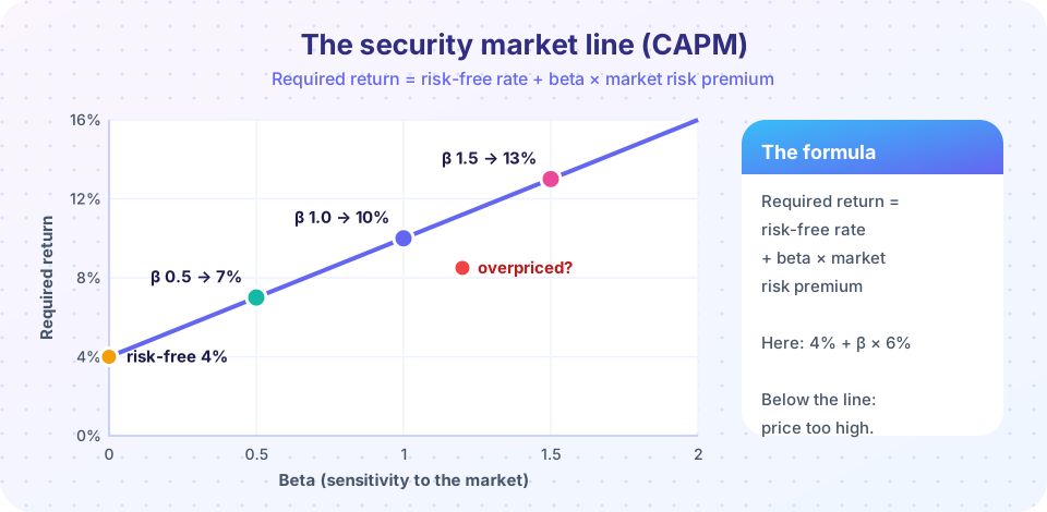
Worked example. Take rf = 4% and an MRP of 6% (so the market's expected return is 10%). Then:
| Asset | Beta | Required return |
|---|---|---|
| Defensive utility | 0.5 | 4% + 0.5 × 6% = 7% |
| The market | 1.0 | 4% + 6% = 10% |
| Aggressive tech | 1.5 | 4% + 9% = 13% |
Notice that required return depends only on beta and the market-wide numbers, not on the asset's own standard deviation.
The security market line and alpha
Plot those three points and they fall on a straight line with intercept rf and slope equal to the MRP: the SML in the picture. The line is the model's prediction of fair expected returns.
Now suppose an analyst believes a stock with β = 1.2 will return 8.5%. The CAPM requires 4% + 1.2 × 6% = 11.2%. The stock's alpha is 8.5% − 11.2% = −2.7%: it plots below the line, offering less than the risk deserves. At today's price it is overpriced; investors would sell it until its price falls enough to lift its expected return onto the line. A stock above the line (positive alpha) is underpriced. In a competitive market, we expect alphas to be close to zero on average, which is why consistent positive alpha is rare and hard to find.
Press Run (or Ctrl + Enter) to see the result here.
Program input · what you'd type while the program runs
Type the answers before you press Run, one per line. Each time the program reads a line (with input()), it gets the next line from this box.
Estimating beta from data
Beta is not directly observable; we estimate it. The standard approach regresses the asset's excess returns (return minus rf) on the market's excess returns, usually with five years of monthly data. The slope is beta. Data providers publish betas, but they differ with the choice of period, return interval and market index. Many practitioners apply an adjustment that pulls estimates toward 1 (a common version is 0.67 × raw + 0.33 × 1), because extreme betas tend to drift back toward the average.
Press Run (or Ctrl + Enter) to see the result here.
Program input · what you'd type while the program runs
Type the answers before you press Run, one per line. Each time the program reads a line (with input()), it gets the next line from this box.
The simulation built in a true beta of 1.30, yet sixty noisy months gave an estimate of about 1.17. That gap is sampling error, and it is a fair picture of real-world betas: they come with a margin of error, so a range of plausible betas is more honest than a single figure. The scatter around the line shows something else important: beta captures only the part of the stock's movement linked to the market. The rest (unique risk) is noise that, as the last lesson showed, diversification removes.
Where the CAPM falls short
An honest treatment lists the cracks.
- One factor. Empirical work by Eugene Fama and Kenneth French found that small companies and "value" companies (low price relative to book value) have earned more than their betas predict. Multi-factor models add size, value, profitability and momentum factors.
- Flat line. In many datasets the actual relationship between beta and return is flatter than the SML: low-beta stocks have earned more than the model says, high-beta stocks less.
- Unstable inputs. Betas move over time, and the MRP is genuinely uncertain: sensible estimates range from about 4% to 7%, which swings the cost of equity by points.
- Unobservable market. The "market portfolio" should include all assets (property, human capital, private business); we use a stock index as a stand-in.
Despite this, the CAPM is used everywhere because it is simple, transparent and gives a defensible starting number. Good practitioners cross-check it against other methods (you will meet them in the next chapter) and treat the result as a range, not a point.
Common misconceptions
"A high-beta stock is a bad stock." Beta is a measure of risk, not quality. A high-beta stock simply needs a high expected return to compensate; if it offers that, it is fairly priced.
"Beta predicts the future." It is estimated from the past and is noisy. Use it as a reasonable input, not a fact.
"A stock with a high standard deviation must have a high beta." Not necessarily. A volatile asset that barely moves with the market has a low beta.
Check your understanding
Quick check · 5 questions
of 5 answered You scored / 5 · perfect!
-
1. With rf = 3% and a market risk premium of 5%, what return does the CAPM require for β = 1.4?
3% + 1.4 × 5% = 3% + 7% = 10.0%. -
2. A stock with β = 0.9 has an expected return of 6% when rf = 3% and the MRP is 5%. What is its alpha?
Required = 3% + 0.9 × 5% = 7.5%. Alpha = 6% − 7.5% = −1.5%, so the stock plots below the SML. -
3. What does a beta of 0 mean?
Beta measures co-movement with the market. A risk-free asset has β = 0, but so can a volatile asset that is uncorrelated with the market. -
4. What is the beta of a portfolio with half in β = 0.6 and half in β = 1.4?
The portfolio beta is the weighted average: 0.5 × 0.6 + 0.5 × 1.4 = 1.0. -
5. Which is a known limitation of the CAPM?
Empirical research by Fama and French found size and value premiums not explained by beta alone.
Summary
- Beta = Cov(asset, market) / Var(market): sensitivity to market moves.
- CAPM: required return = rf + β × market risk premium.
- The SML plots required return against beta; assets below the line are overpriced.
- Beta is estimated by regression and is noisy; the CAPM is a useful but imperfect single-factor model.
Next: Chapter review
Track your progress
Create a free account to tick off lessons and pick up where you left off on any device.
of Corporate Finance lessons completed