


















Lesson 18 of 46 · Free Electron Model
Density of states and electronic heat capacity
Derive the free electron density of states g(E) ∝ √E, use the Fermi-Dirac distribution, and get the linear electronic heat capacity C = γT for copper and other metals.
How many electronic states are there between energy E and E + dE? That count, the density of states g(E), appears in nearly every calculation in condensed matter physics: heat capacity, conductivity, optical absorption, magnetism and the behavior of semiconductors. For free electrons it is a simple curve, and with it we can resolve the paradox of Drude's electron heat capacity.
You will see that only electrons within about k_BT of the Fermi energy can absorb heat, and from that picture derive the observed linear-in-T heat capacity.
What you will learn
- How to derive g(E) for three-dimensional free electrons.
- How the Fermi-Dirac distribution describes occupation at finite temperature.
- How to obtain the electronic heat capacity C = γT and the coefficient γ.
- How measured γ values reveal electron interactions (thermal effective mass).
Key terms
Density of states g(E): the number of one-electron states per unit energy (and per unit volume if divided by V).
Fermi-Dirac distribution: f(E) = 1/(e^{(E − μ)/k_BT} + 1), the probability that a state of energy E is occupied.
Chemical potential μ: the energy at which f = 1/2; μ = E_F at T = 0 and μ ≈ E_F at ordinary temperatures.
Sommerfeld coefficient γ: the slope of the electronic heat capacity, C_el = γT.
Density of states in three dimensions
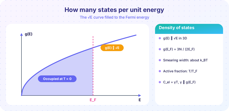
Start from the number of states with energy below E. A free electron has E = ħ²k²/2m, so the states below E fill a sphere of radius k = (2mE)^(1/2)/ħ. With spin degeneracy, the count is
N(E) = 2 × (4π k³/3) / (2π/L)³ = V k³/(3π²) = (V/3π²)(2mE/ħ²)^(3/2).
Differentiating gives the density of states:
g(E) = dN/dE = (V/2π²) (2m/ħ²)^(3/2) √E.
Three observations. First, g(E) ∝ √E: higher energy means a larger sphere shell and more states. Second, since N = (V/3π²)(2mE_F/ħ²)^(3/2) at the Fermi energy, dividing gives a neat relation, g(E_F) = 3N/(2E_F). Third, in lower dimensions the shape changes: g(E) is constant in 2D and ∝ 1/√E in 1D, which is why quantum wells and nanowires behave differently.
The Fermi-Dirac distribution
At temperature T the probability that a state of energy E is occupied is
f(E) = 1 / ( e^{(E − μ)/k_BT} + 1 ).
At T = 0 it is a step: 1 for E < μ and 0 for E > μ. At finite T the step is rounded over an energy range of about 4k_BT centered on μ. For a metal at 300 K that is about 0.1 eV, compared with E_F of several eV. The chemical potential shifts only slightly with T: μ ≈ E_F[1 − (π²/12)(T/T_F)²], a correction of order 10⁻⁵ at room temperature, so we can set μ = E_F.
The number of electrons per energy interval is g(E) f(E). To change the energy of the gas you must move electrons from filled states to empty ones near the edge.
Why the heat capacity is small and linear
Raise the temperature from 0 to T. Only electrons in a shell of thickness of order k_BT below E_F can gain energy of order k_BT, as the rest have no empty states to move to. The number of such electrons is about g(E_F) k_BT, and each gains about k_BT, so the extra energy is about g(E_F)(k_BT)² and the heat capacity is proportional to T. The careful evaluation by Sommerfeld gives
U − U₀ = (π²/6) g(E_F) (k_BT)² and C_el = dU/dT = (π²/3) g(E_F) k_B² T = γ T.
Using g(E_F) = 3N/(2E_F) and T_F = E_F/k_B:
C_el = (π²/2) N k_B (T/T_F).
Compare it with the classical 3Nk_B/2: the electrons contribute a fraction (π²/3)(T/T_F) of it, about 1% at room temperature. For one mole of copper at 300 K, T/T_F = 0.0037, so C_el = 4.93 × 8.314 × 0.0037 ≈ 0.15 J/(mol·K), small against the lattice's 24 J/(mol·K).
At room temperature the lattice term dominates, so we only see the electrons at very low temperature. The total heat capacity is
C = γ T + β T³
where the cubic term is the Debye phonon contribution (Lesson 340). Plotting C/T against T² yields a straight line whose intercept is γ and whose slope is β. The crossover, where γT = βT³, is at about T = √(γ/β), roughly 4 K for copper.
Comparing with experiment
For copper the free-electron value is γ = π²R/(2T_F) = 0.505 mJ/(mol·K²), while the measured value is 0.695 mJ/(mol·K²). The ratio gives the thermal effective mass:
m*/m = γ_measured / γ_free
so copper's m* ≈ 1.38 m. For sodium it is 1.26, aluminum 1.48 and potassium 1.25. The electrons respond as if heavier than free electrons, because they interact with the lattice (the band structure of Chapter 5) and with phonons and each other. The model is quantitatively imperfect but qualitatively right, a very good score for a theory that ignores most of the physics. Dramatic exceptions exist: in "heavy fermion" compounds m* reaches hundreds of electron masses.
Common misconceptions
"All electrons absorb heat." Only a fraction of order T/T_F do. The rest are frozen into the Fermi sea.
"The electronic term is visible at room temperature." The phonon term is more than a hundred times larger at 300 K in copper; the electronic γT shows up clearly only below about 10 K.
"A larger γ means more electrons." γ ∝ g(E_F) ∝ m* n^(1/3): it measures the density of states at the Fermi level, which increases with effective mass as well as electron number.
Try it
Press Run (or Ctrl + Enter) to see the result here.
Program input · what you'd type while the program runs
Type the answers before you press Run, one per line. Each time the program reads a line (with input()), it gets the next line from this box.
Press Run (or Ctrl + Enter) to see the result here.
Program input · what you'd type while the program runs
Type the answers before you press Run, one per line. Each time the program reads a line (with input()), it gets the next line from this box.
Check your understanding
Quick check · 5 questions
of 5 answered You scored / 5 · perfect!
-
1. The density of states of free electrons in 3D is proportional to
g(E) ∝ √E, because the sphere of states grows as k³ ∝ E^(3/2). -
2. What is g(E_F) in terms of N and E_F?
From N ∝ E_F^(3/2), g = dN/dE = (3/2)N/E_F. -
3. At low T the electronic heat capacity is
Only electrons within about k_BT of E_F can be excited; their number is proportional to T and each gains about k_BT. -
4. Plotting C/T against T² for a metal gives a straight line whose intercept is
C/T = γ + βT², so the intercept at T² = 0 is the electronic coefficient γ. -
5. Copper has γ_measured = 0.695 and γ_free = 0.505 mJ/(mol·K²). What is its thermal effective mass ratio?
0.695/0.505 = 1.376.
Summary
- g(E) = (V/2π²)(2m/ħ²)^(3/2)√E and g(E_F) = 3N/(2E_F).
- f(E) is a step at T = 0 and rounded over about 4k_BT otherwise; μ ≈ E_F.
- Only a fraction of order T/T_F of electrons can absorb heat, so C_el = (π²/3)g(E_F)k_B²T = γT.
- Measured γ exceeds the free-electron value by a factor m*/m of order 1.2 to 1.5 in simple metals.
- Low-temperature data are analyzed with C/T = γ + βT².
Track your progress
Create a free account to tick off lessons and pick up where you left off on any device.
of Condensed Matter Physics lessons completed