


















Lesson 12 of 45 · Sampling and Calibration
Sampling heterogeneous materials
Understand sampling error, why heterogeneous solids need large samples, how mixing, splitting and grinding help, and how to estimate the sample mass you need.
Imagine a 20-tonne load of ore in which 1 particle in 1,000 is rich in gold. You take a 5 g scoop. How many rich particles are in it? Probably none, or one. The assay will say "no gold" or "a lot of gold", and neither describes the load. This is sampling error, and it is the reason a careful analyst thinks about the sample before thinking about the instrument.
What you will learn
- Distinguish population, gross sample, laboratory sample and analysis portion.
- Use the binomial model to estimate the sampling uncertainty from rare particles.
- Apply the Ingamells sampling constant to choose a sample mass.
- Reduce the sample size correctly with mixing, grinding, coning and quartering, and riffle splitting.
Key terms
Population (lot): the whole material you want to describe. Gross sample: the combined increments collected from the lot. Laboratory sample: the portion delivered to the lab after reduction. Analysis portion (test portion): the amount actually measured. Heterogeneity: variation in composition between parts of the material.
Sampling plans
A representative sample is one in which every part of the lot had a chance to be chosen and the analyte proportion is preserved. Practical plans:
- Random sampling gives each part an equal chance (use random numbers, not "wherever it is convenient").
- Stratified sampling divides the lot into layers or zones (depth of a lake, top and bottom of a truck) and samples each.
- Composite sampling blends many increments into one gross sample, averaging out local variation.
- Systematic sampling samples at regular intervals, useful for flowing streams, but beware periodic patterns in the process.
For liquids, mix first if the lot is homogeneous, and collect in clean containers appropriate for the analyte (acid-washed plastic for trace metals; glass for organics). For gases, flow, volume and time matter. Always preserve the sample (cooling, acidifying, adding stabilizers) so it does not change between collection and analysis, and label it with date, place and collector.
Particles and the binomial model
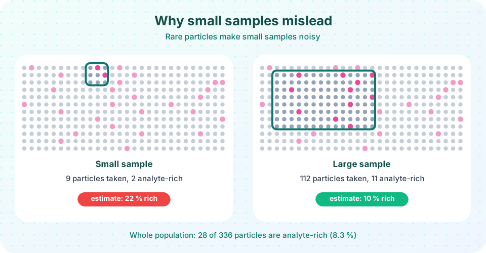
Suppose a fraction p of the particles carries the analyte and you take n particles at random. The number of analyte-rich particles in the sample is binomially distributed: mean n p, standard deviation √(n p (1 − p)). The relative standard deviation of the count is
RSD = √( (1 − p) / (n p) )
Take p = 0.10: a sample of 100 particles holds 10 on average with RSD = √(0.9/10) = 0.30 = 30 %. To get 5 % you need n p ≈ 360, i.e. n ≈ 3,600 particles. A tenfold smaller p needs ten times as many. Rare things need big samples.
The Ingamells sampling constant
Real particles vary in size and composition, so a more convenient empirical relation is
w R² = K_s
where w is the sample mass in grams, R the relative standard deviation due to sampling in percent, and K_s the sampling constant (the mass needed for a 1 % RSD), determined by measuring several samples of different mass. If K_s = 20 g: a 1 g sample has R = √(20/1) = 4.5 %; to reach R = 1 % you need 20 g; to reach 0.5 % you need 80 g. The cost of precision rises quickly.
Reducing the sample
You cannot grind a tonne of rock to a milligram in one step, nor can you analyze it whole. The standard route:
- Collect a large, composite gross sample.
- Crush and grind so particles are small: the number of particles per gram rises sharply with fineness, reducing the sampling error.
- Mix thoroughly, then split without bias: riffle splitters, rotary dividers, or coning and quartering (pile in a cone, flatten, divide into four, keep opposite quarters).
- Repeat grind-and-split until you have the laboratory sample, then weigh the analysis portion.
A rule of thumb: the sample mass should shrink in step with particle size, never faster. Splitting a coarse sample to a tiny mass leaves too few particles; a stage-by-stage plan that grinds finer before every split keeps the relative error constant.
Sample variance adds
Sampling and analysis variances add: s_total² = s_sampling² + s_analysis². If you find that the total variance of results from different portions is much bigger than the variance of repeated analyses of one well-mixed portion, sampling is the problem. Then more replicates of the analysis do nothing: take more or bigger samples.
Common misconceptions
"Any scoop is a sample." Convenient scoops are biased toward the surface and the easy-to-reach part.
"Double the replicates fixes the scatter." If sampling dominates, extra analytical replicates of the same portion do not help.
"Grind less to save time." Coarse particles mean few particles per sample and a large sampling error.
Try it
Press Run (or Ctrl + Enter) to see the result here.
Program input · what you'd type while the program runs
Type the answers before you press Run, one per line. Each time the program reads a line (with input()), it gets the next line from this box.
Press Run (or Ctrl + Enter) to see the console output here.
No output.
Check your understanding
Quick check · 5 questions
of 5 answered You scored / 5 · perfect!
-
1. Which part of a sampling hierarchy is the largest?
The lot is the whole material; the gross sample, laboratory sample and analysis portion are successively smaller. -
2. With p = 0.10 and n = 100 particles, the sampling RSD is
√((1 − 0.10)/(100 × 0.10)) = √0.09 = 0.30. -
3. K_s = 20 g. Which sample mass gives a sampling RSD of 2 %?
w = K_s/R² = 20/4 = 5 g. -
4. Grinding a coarse sample finer before splitting helps because
More, smaller particles per gram mean the binomial sampling error shrinks. -
5. Total variance of results is much larger than the variance from replicate analyses of one portion. The main problem is
Between-portion variance is sampling variance.
Summary
- A sample must represent the lot: use random, stratified or composite plans.
- Rare analyte-rich particles demand many particles per sample;
RSD = √((1−p)/(np)). - The Ingamells constant
wR² = K_slinks sample mass to sampling error. - Reduce samples by grinding and splitting in stages; preserve and label them.
Track your progress
Create a free account to tick off lessons and pick up where you left off on any device.
of Analytical Chemistry lessons completed