


















Lesson 24 of 45 · Electrochemical Analysis
Voltammetry, conductometry and coulometry
Understand cyclic voltammetry, stripping analysis, conductometric titrations and Faraday's law of coulometry, with worked numbers and runnable simulations.
Potentiometry is passive: it reads a voltage and disturbs nothing. The other electrochemical methods are active. They apply a potential or a current and watch how the cell reacts. That extra control makes them far more sensitive, and in the case of coulometry, absolute.
This lesson covers three families. In voltammetry you scan the potential and measure the current. In conductometry you measure how well ions carry a current. In coulometry you count the electrons that pass.
What you will learn
- Describe the three-electrode cell and why a supporting electrolyte is used.
- Read a cyclic voltammogram and apply the Randles–Ševčík equation.
- Explain stripping voltammetry and why it reaches such low detection limits.
- Plan a conductometric titration and sketch its V-shaped curve.
- Use Faraday's law to turn charge into moles and mass.
Key terms
Working electrode: where the reaction of interest happens; its potential is controlled.
Counter electrode: completes the circuit and carries the current.
Supporting electrolyte: a high concentration of inert salt that suppresses migration and lowers solution resistance.
Diffusion-limited current: a current set by how fast analyte reaches the electrode, not by the reaction speed.
Faraday constant: 96,485 C of charge per mole of electrons.
Voltammetry: scan, then measure
The three-electrode cell
A potentiostat controls the potential of the working electrode (glassy carbon, platinum, gold or a mercury film) against a reference electrode, and sends the current through a counter electrode such as a platinum wire. Keeping the current away from the reference electrode protects its potential. The solution contains the analyte plus 0.1 M or more of supporting electrolyte, for example KCl or a buffer. The electrolyte carries the current in solution so that the analyte moves to the electrode by diffusion only, not by electrical migration.
Why a peak appears
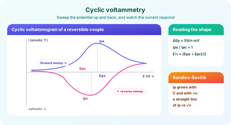
Take a species R that is oxidized to O at the working electrode. At a potential far below E°, nothing happens. As the potential rises, R at the surface is oxidized, a gradient forms, and current climbs. But the layer next to the electrode runs out of R, so the diffusion layer thickens and the current falls again. The result is a peak, then a decay that follows t^(−1/2).
For a reversible couple the peak current is given by the Randles–Ševčík equation (25 °C):
ip = 2.69 × 10⁵ · n^(3/2) · A · D^(1/2) · C · v^(1/2)
with ip in amperes, n electrons, A in cm², D in cm²/s, C in mol/cm³ and the scan rate v in V/s. So the peak current is linear in concentration (the basis of analysis) and in the square root of scan rate (a test for a diffusion-controlled process).
Reading the voltammogram
In cyclic voltammetry the potential sweeps up, reverses, and returns. For a fast reversible couple:
- the peak separation is
ΔEp = Epa − Epc ≈ 59/n mVat 25 °C; - the ratio of peak currents is
ipa / ipc ≈ 1; - the formal potential is
E°′ ≈ (Epa + Epc)/2.
A larger separation signals a slow electron transfer or uncompensated resistance. A missing reverse peak signals that the product reacts further.
Press Run (or Ctrl + Enter) to see the result here.
Program input · what you'd type while the program runs
Type the answers before you press Run, one per line. Each time the program reads a line (with input()), it gets the next line from this box.
A simulated cyclic voltammogram
The following code solves Fick's second law by finite differences for a Nernstian (reversible) couple. It is a simulation: it applies the model, with no experiment behind it. Starting with only R present, the potential is swept from 257 mV below E°′ to 257 mV above it and back (dimensionless values ±10 RT/F).
Press Run (or Ctrl + Enter) to see the result here.
Program input · what you'd type while the program runs
Type the answers before you press Run, one per line. Each time the program reads a line (with input()), it gets the next line from this box.
Stripping analysis
Standard voltammetry reaches about 10⁻⁵ to 10⁻⁶ M. Anodic stripping voltammetry (ASV) goes much lower by cheating on concentration. First, the electrode is held at a negative potential for a few minutes while stirring, and metal ions such as Pb²⁺, Cd²⁺ and Zn²⁺ are reduced and preconcentrated into a mercury film or onto a bismuth or carbon surface. After a rest, the potential is scanned positively. Each metal is stripped back into solution at its own potential, giving a sharp peak whose height is proportional to the concentration. Detection limits reach the µg/L range and below. Quantification is usually by the method of standard additions, which you will meet in Chapter 3.
Amperometry and biosensors
If the potential is held constant and the current is monitored, the technique is amperometry. The Clark oxygen electrode reduces dissolved oxygen at a platinum cathode behind a gas-permeable membrane. The glucose biosensor combines the enzyme glucose oxidase with an electrode: the enzymatic product is detected as a current proportional to the amount of glucose.
Conductometry
Every ion carries current. The conductivity of a dilute solution is the sum over all ions:
κ = Σ λᵢ · cᵢ (with κ in S/cm, c in mol/cm³, λ in S cm²/mol)
Limiting molar conductivities at 25 °C, in S cm²/mol, are about: H⁺ 349.8, OH⁻ 198, Na⁺ 50.1, K⁺ 73.5, Cl⁻ 76.3 and acetate 40.9. Hydrogen and hydroxide are exceptional because protons hop along the water network.
Conductivity is not selective, so direct measurements are mostly used for water purity and total dissolved salts. But in a conductometric titration it is excellent. In HCl titrated with NaOH, fast H⁺ is replaced by slower Na⁺, so the conductivity falls. After the equivalence point, the extra OH⁻ makes it rise. The end point is the minimum, found as the intersection of two straight lines.
Press Run (or Ctrl + Enter) to see the result here.
Program input · what you'd type while the program runs
Type the answers before you press Run, one per line. Each time the program reads a line (with input()), it gets the next line from this box.
Coulometry: counting electrons
Michael Faraday showed that the amount of substance changed at an electrode is proportional to the charge that passes. For a reaction involving n electrons per particle,
N = Q / (n F) and m = (i · t · M) / (n F)
where Q = i·t is the charge in coulombs, F = 96,485 C/mol, and M is the molar mass. The method is absolute: no calibration curve is needed, as long as the reaction goes with 100 % current efficiency, meaning every electron does the intended job and nothing else.
Worked example. A constant current of 50.0 mA passes for 600 s while copper deposits from Cu²⁺ (n = 2). Q = 0.0500 × 600 = 30.0 C. N = 30.0 / (2 × 96,485) = 1.555 × 10⁻⁴ mol. With M = 63.55 g/mol this is 9.88 mg of copper.
Two modes exist. Controlled-potential (bulk electrolysis) coulometry holds the potential of the working electrode and integrates the current until it decays to near zero. Constant-current coulometric titration generates the titrant at the electrode: you measure time instead of volume, and time is the easiest quantity to measure accurately.
The best known example is Karl Fischer titration for water. Iodine is generated at the anode; each molecule of iodine consumes one water molecule in the reaction with sulfur dioxide, a base and an alcohol. One mole of water needs one mole of iodine, which is 2 F, so 1 mg of water corresponds to 10.71 C.
Press Run (or Ctrl + Enter) to see the result here.
Program input · what you'd type while the program runs
Type the answers before you press Run, one per line. Each time the program reads a line (with input()), it gets the next line from this box.
Common misconceptions
"More current always means more analyte." In voltammetry the current is limited by diffusion, so it depends on scan rate and electrode area as well as concentration. Compare like with like.
"Dissolved oxygen is harmless." Oxygen is reduced at around −0.1 to −0.9 V and produces large background waves. Purge with nitrogen or argon before scanning to negative potentials.
"Coulometry is always 100 % efficient." Side reactions (for example, water splitting) waste charge. Always check the current efficiency.
Check your understanding
Quick check · 5 questions
of 5 answered You scored / 5 · perfect!
-
1. Why is a high concentration of supporting electrolyte added in voltammetry?
An excess of inert ions carries most of the current, so the analyte moves by diffusion. It also reduces the ohmic drop. -
2. In a reversible cyclic voltammogram with n = 1, what peak separation is expected at 25 °C?
For a reversible one-electron couple, the peak separation is roughly 59/n mV. -
3. What does a plot of ip against the square root of scan rate that is linear and passes through the origin suggest?
Randles–Ševčík predicts ip proportional to sqrt(v) when diffusion controls the current. -
4. A 100 mA current flows for 965 s with 100 % efficiency in a one-electron reaction. How many moles react?
Q = 0.100 A × 965 s = 96.5 C, and N = 96.5 / 96,485 = 1.0 × 10⁻³ mol. -
5. Why does the conductivity fall during the first part of an HCl/NaOH conductometric titration?
H+ has a much higher molar conductivity than Na+. Neutralization swaps the former for the latter.
Summary
- Voltammetry applies a potential scan and measures current; the peak current is proportional to concentration and to √v for diffusion control.
- A reversible CV has
ΔEp ≈ 59/n mV,ipa/ipc ≈ 1andE°′midway between the peaks. - Stripping voltammetry preconcentrates metals first, reaching trace levels.
- Conductometric titrations give V-shaped or L-shaped curves; the end point is the intersection of straight segments.
- Faraday's law,
N = Q/(nF), makes coulometry an absolute method; Karl Fischer needs 10.71 C per mg of water.
Next: Chapter 5 review
Track your progress
Create a free account to tick off lessons and pick up where you left off on any device.
of Analytical Chemistry lessons completed