


















Lesson 13 of 45 · Sampling and Calibration
Calibration curves and detection limits
Build an external calibration curve by least squares, use it to find an unknown with its uncertainty, check residuals and calculate the LOD and LOQ.
An instrument does not report grams per liter. It reports a signal: an absorbance, a peak area, a current. A calibration is the bridge between the two. You measure standards of known concentration, draw the best line through the points, and use that line backward to turn an unknown's signal into a concentration. This lesson shows how to do that properly, and how to say how small an amount the method can reliably detect.
What you will learn
- Fit a straight line by least squares and interpret slope and intercept.
- Calculate an unknown concentration and judge its uncertainty.
- Check linearity with residuals instead of relying on r² alone.
- Define and compute the limit of detection (LOD) and limit of quantification (LOQ).
Key terms
Calibration curve: signal plotted against standard concentration. Sensitivity: the slope m of the calibration line. Linear range: the concentrations over which the response is a straight line. Residual: observed signal minus the signal predicted by the line. Blank: a sample with no analyte, carried through the whole procedure.
External calibration
Prepare at least five standards that bracket the expected concentration (the unknown should fall in the middle, not beyond the highest standard), measure them in random order together with a blank, and fit
y = m x + b
with y the signal and x the concentration. The least-squares estimates are
m = Σ(x_i − x̄)(y_i − ȳ) / Σ(x_i − x̄)² and b = ȳ − m x̄.
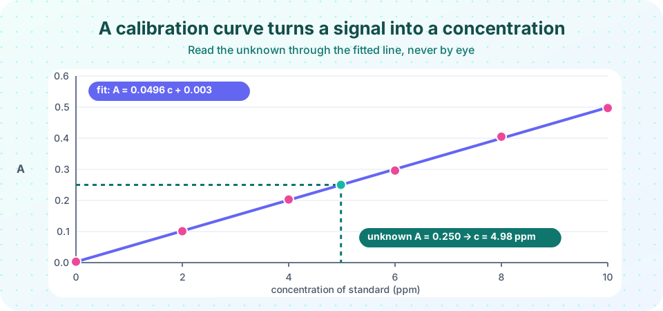
For the six points in the figure (0, 2, 4, 6, 8, 10 ppm with absorbances 0.003, 0.101, 0.203, 0.296, 0.405, 0.497) the fit gives m ≈ 0.0496 ppm⁻¹ and b ≈ 0.003. An unknown with A = 0.250 then has x = (0.250 − 0.003)/0.0496 ≈ 4.98 ppm. Remember to multiply by any dilution factor applied to the sample.
Uncertainty of the result
The scatter of the points about the line is s_y/x = √( Σ residual² / (n − 2) ). The standard uncertainty of an unknown found from m_u replicate readings is
s_x = (s_y/x / m) × √( 1/m_u + 1/n + (y_u − ȳ)² / (m² Σ(x_i − x̄)²) )
The last term grows as the unknown moves away from the center of the calibration; so the best accuracy is in the middle of the range. More standards and more replicates of the unknown narrow the interval.
Is it really a straight line?
A correlation coefficient close to 1 does not prove linearity: a curved response can still have r² = 0.998. Plot the residuals: they should scatter randomly around zero. A systematic pattern (a U shape or a trend) means the line is wrong. Do not extrapolate beyond the highest standard, and do not force the line through zero unless the blank shows the intercept is not significantly different from zero.
Detection and quantification limits
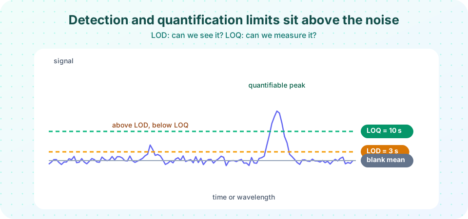
How small an amount can the method tell from noise? Measure the blank at least ten times and find its standard deviation s_blank. Then (using the IUPAC-style convention)
- LOD = 3 s_blank / m: the smallest concentration whose signal is distinguishable from the blank noise.
- LOQ = 10 s_blank / m: the smallest concentration that can be measured with acceptable precision (about 10 % RSD).
The ICH guideline for pharmaceutical methods uses the slope and the residual standard deviation, LOD = 3.3 σ/m and LOQ = 10 σ/m, where σ is s_y/x or the standard deviation of the intercept. Report which convention you used.
Common misconceptions
"r² = 0.999 proves the calibration is good." It does not detect curvature or a poor fit at the low end. Check the residuals.
"Extend the line to the unknown." An unknown above the top standard needs dilution or a new standard, not extrapolation.
"LOD is the instrument's lowest reading." It depends on the whole method and its blank, not just the display.
Try it
Press Run (or Ctrl + Enter) to see the result here.
Program input · what you'd type while the program runs
Type the answers before you press Run, one per line. Each time the program reads a line (with input()), it gets the next line from this box.
Press Run (or Ctrl + Enter) to see the result here.
Program input · what you'd type while the program runs
Type the answers before you press Run, one per line. Each time the program reads a line (with input()), it gets the next line from this box.
Check your understanding
Quick check · 5 questions
of 5 answered You scored / 5 · perfect!
-
1. In y = m x + b for a calibration, the slope m is called the
The change in signal per unit concentration is the calibration sensitivity. -
2. A calibration line is y = 0.050 x + 0.004 (x in ppm). An unknown gives y = 0.254. Its concentration is
x = (0.254 − 0.004)/0.050 = 5.0 ppm. -
3. A residual plot shows a clear U-shaped pattern. This means
Random residuals support a straight line; a systematic curve indicates curvature. -
4. s_blank = 0.0010 and m = 0.050 per ppm. The LOD (3 s/m) is
3 × 0.0010 / 0.050 = 0.060 ppm. -
5. Where in the calibration range is the uncertainty of an unknown smallest?
The term (y_u − ȳ)² is zero at the mean signal, so the interval is narrowest in the middle.
Summary
- Fit signal against concentration by least squares, bracket the unknown and do not extrapolate.
- Check residuals, not only r².
- LOD ≈ 3 s_blank/m and LOQ ≈ 10 s_blank/m; a bigger slope lowers both.
Track your progress
Create a free account to tick off lessons and pick up where you left off on any device.
of Analytical Chemistry lessons completed