


















Lesson 14 of 46 · Smith Chart and Matching
Stub and Quarter-Wave Matching
Design single-stub and quarter-wave matches step by step: stub position and length from the admittance equation, numeric worked examples and a designer you can run.
At microwave frequencies lumped inductors and capacitors become unreliable: they have parasitics, tolerances and low Q. Printed transmission lines on the board, on the other hand, are cheap and accurate. That is why microwave matching networks are built from line pieces: a quarter-wave section to step between two resistances, or a stub (a short branch of line) placed at the right distance from the load to cancel the reactance.
This lesson shows how both methods work, gives the exact design equations for the single-stub match and compares their bandwidths.
What you will learn
- When the quarter-wave transformer works, and its bandwidth.
- The idea of the single-stub match: move to where
Re(y) = 1, then cancel the susceptance with a stub. - How to compute the stub distance and length numerically.
- Differences between shorted and open stubs and between series and shunt stubs.
Key terms
- Admittance (y):
y = 1/z, normalized to1/Z0;y = g + jb. - Susceptance (b): the imaginary part of admittance.
- Shunt stub: a stub connected in parallel with the main line.
- Stub position (d): distance from the load to the stub junction.
- Stub length (l): electrical length of the stub itself.
The quarter-wave transformer in practice
From the previous chapter, Z1 = √(Z0 · RL) matches a real load RL to Z0. Three practical points:
- Real loads only. If the load has reactance, first cancel it or move along the line to a point where the impedance is real. At the point on the line where the voltage is at a maximum (or minimum) the impedance is a pure resistance,
Z0 · VSWR(orZ0 / VSWR), so a transformer placed there works. - Realizable impedances. On microstrip, impedances from about 20 Ω to 120 Ω are practical. Very high ratios need unrealistically narrow or wide lines.
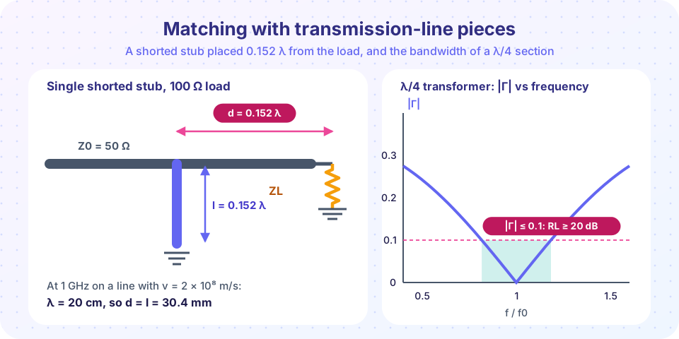
- Bandwidth. The reflection stays below 0.1 (return loss better than 20 dB) from about 0.82 to 1.18 times the design frequency when matching 100 Ω to 50 Ω; for 200 Ω to 50 Ω it is 0.915 to 1.085 times (these numbers come from the simulation in the previous lesson).
The single-stub match
For a general complex load, a single shunt stub gives a match using two design numbers: where to place it and how long to make it. The idea works in admittance because shunt elements add admittances.
- Write the load as a normalized admittance
yL = g + jb. - Move a distance
dtoward the generator until the real part of the admittance reaches 1:y(d) = 1 + jb'. (On the Smith chart, this is the intersection of the load's VSWR circle with theg = 1circle.) - Add a stub with susceptance
−jb'. The total is1 + j0: matched.
The admittance of a lossless line section is y(d) = (yL + j t)/(1 + j yL t) with t = tan βd. Setting Re y = 1 gives a quadratic in t:
(g − g² − b²) t² + 2b t + (g − 1) = 0
It usually has two solutions, so there are two possible positions. For each, compute b' = Im y(d):
- A shorted stub has
b = −cot βl, so choosecot βl = b'. - An open stub has
b = +tan βl, so choosetan βl = −b'.
Worked example: 100 Ω load on 50 Ω
yL = 50/100 = 0.5(sog = 0.5,b = 0).- The quadratic reduces to
0.25 t² − 0.5 = 0, sot = ±√2 = ±1.414. - Take
t = +1.414:βd = arctan(1.414) = 54.74°,d = 54.74/360 = 0.152 λ. - At that point
y = (0.5 + j1.414)/(1 + j0.707) = 1 + j0.707. Sob' = 0.707. - A shorted stub needs
cot βl = 0.707, sotan βl = 1.414,βl = 54.74°andl = 0.152 λ.
(The matching numbers d = l = 0.152 λ are a coincidence for this load. For other loads the two differ.)
At 1 GHz on a line with velocity factor 0.667 (λ = 20 cm), d = l = 30.4 mm.
The other solution, t = −1.414, gives d = 0.348 λ and a shorted stub 0.348 λ long. It is the mirror image of the first, but both the line and the stub are longer.
Shorted or open?
Both do the job; pick one for practical reasons:
- Open stubs in microstrip are easy: no via to ground. But an open end radiates a little and its fringing field makes it electrically slightly longer than it looks; compensate by shortening it.
- Shorted stubs in coax and waveguide are common because a shorted line does not radiate and a metal slug is easy to slide.
- The shorter solution of the two is usually better since longer stubs are more narrowband.
Series stubs and double stubs
A series stub puts the reactive element in series with the line instead of in parallel: it needs a break in the conductor, which is awkward on microstrip but easy on balanced lines. Double-stub tuners use two stubs at fixed spacing so only their lengths change; they can match many loads but not all. A triple-stub tuner can match any load.
Bandwidth
Stubs are narrowband because both the line length and the stub's own length vary with frequency. For the 100 Ω load, the simulation below shows the quarter-wave transformer keeping |Γ| ≤ 0.1 from 0.818 to 1.183 times the design frequency, while the single shorted stub manages 0.921 to 1.094: about half as wide. The program plots both so you can compare them.
Common misconceptions
- "The stub length equals the amount of reactance to cancel." The stub cancels the susceptance after you have moved to the point where
g = 1. Its length comes fromcot βl = b', not from the original load reactance. - "A quarter-wave stub is always 90°." A quarter-wave stub is
λ/4long (90°); the stubs in matching networks are usually much shorter, between 0 andλ/2. - "Open and short are interchangeable lengths." They differ by
λ/4: if a shorted stub of lengthlworks, an open stub of lengthl + λ/4does as well.
Try it
This designer finds both stub positions for any complex load and checks the result by adding the stub admittance and recomputing the reflection. The first row is the worked example above.
Press Run (or Ctrl + Enter) to see the result here.
Program input · what you'd type while the program runs
Type the answers before you press Run, one per line. Each time the program reads a line (with input()), it gets the next line from this box.
Second, the bandwidth comparison. It sweeps frequency for a 100 Ω load matched by a quarter-wave section and by the shunt-stub design above.
Press Run (or Ctrl + Enter) to see the result here.
Program input · what you'd type while the program runs
Type the answers before you press Run, one per line. Each time the program reads a line (with input()), it gets the next line from this box.
Check your understanding
Quick check · 5 questions
of 5 answered You scored / 5 · perfect!
-
1. A quarter-wave transformer matches which kind of load to Z0?
The transformer relation Zin = Z1²/RL holds for a real load. -
2. In the single-stub method, the stub is placed where
At that point the normalized admittance is 1 + jb', and the stub cancels jb'. -
3. A shorted stub of length l has normalized susceptance
A shorted stub is jZ0 tan βl in impedance, so −j cot βl in admittance. -
4. Why are stubs and quarter-wave sections common above a few GHz?
Lines are defined by lithography; small inductors and capacitors have parasitics and low Q. -
5. For the 100 Ω example, what is the stub position d?
tan βd = 1.414 gives βd = 54.7°, d = 0.152 λ (a second solution is 0.348 λ).
Summary
- Quarter-wave transformers match real loads with
Z1 = √(Z0 RL). - The single-stub method: move to
Re(y) = 1, then cancel the susceptance with a stub. - Position:
(g − g² − b²) t² + 2bt + (g − 1) = 0; shorted stub:cot βl = b'; open stub:tan βl = −b'. - The 100 Ω load needs
d = l = 0.152 λ(30.4 mm at 1 GHz in 0.667 VF line). - Both methods are narrowband; use multiple sections or lumped parts for wider bands.
Next: Chapter 3 Review
Track your progress
Create a free account to tick off lessons and pick up where you left off on any device.
of RF Engineering and Antennas lessons completed