


















Lesson 15 of 46 · Smith Chart and Matching
Chapter 3 Review: Smith Chart and Matching
Review chapter 3: reading the Smith chart, moving along lines, L-network design, single-stub and quarter-wave matching, with practice problems and a ten-question quiz.
Chapter 3 turned the algebra of chapter 2 into pictures and recipes. You learned that every passive impedance is a point on the Smith chart, that a transmission line rotates that point and that matching networks are paths back to the center. This review pulls the toolbox together and tests whether you can pick the right tool for a given problem.
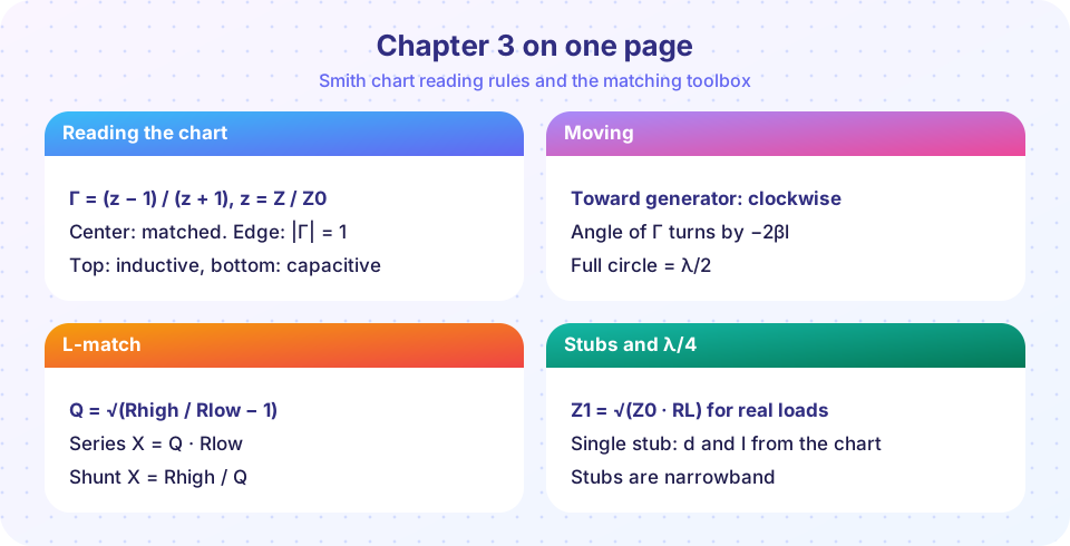
The chapter in a table
| Topic | Key facts |
|---|---|
| Normalization | z = Z/Z0, Γ = (z − 1)/(z + 1) |
| Chart layout | Center = match, left = short, right = open, upper = inductive, lower = capacitive |
| VSWR | Read r where the VSWR circle crosses the real axis on the right |
| Along a line | Clockwise toward the generator; λ/2 per turn; λ/4 gives 1/z |
| Series part | Moves along a constant-r circle (L clockwise, C counter-clockwise) |
| Shunt part | Moves along a constant-g circle (C clockwise, L counter-clockwise) |
| L-match | Q = √(Rhigh/Rlow − 1), Xs = Q Rlow, Xp = Rhigh/Q; shunt across the higher R |
| Quarter-wave | Z1 = √(Z0 RL), real loads only |
| Single stub | Move to Re(y) = 1, cancel jb' with a stub of length cot βl = b' (short) or tan βl = −b' (open) |
Choosing a method
Real load, one frequency
Simplest choices.
Complex load
Cancel the reactance.
Wider band
More parts, more bandwidth.
Start every matching problem by sketching the Smith chart path in your head: where is the load, where is the goal and which moves (series, shunt, line) walk you there?
Try it
Practice problems are solved by code. Solve each by hand first.
Press Run (or Ctrl + Enter) to see the result here.
Program input · what you'd type while the program runs
Type the answers before you press Run, one per line. Each time the program reads a line (with input()), it gets the next line from this box.
Finally, a summary plot of all three matching techniques for the same 100 Ω load. The curve for each is |Γ| against frequency; the dashed line marks 20 dB return loss.
Press Run (or Ctrl + Enter) to see the result here.
Program input · what you'd type while the program runs
Type the answers before you press Run, one per line. Each time the program reads a line (with input()), it gets the next line from this box.
Check your understanding
Quick check · 10 questions
of 10 answered You scored / 10 · perfect!
-
1. A load of 75 + j0 Ω on a 50 Ω system normalizes to
z = 75/50 = 1.5. -
2. Where does the circle r = 1 cross the real axis on the right?
Every constant-r circle touches Γ = +1. The r = 1 circle also passes through the center z = 1. -
3. You move a load 0.25 λ toward the generator. Its new normalized impedance is
A quarter wave is a half turn on the chart: z becomes 1/z. -
4. A shunt capacitor moves a point on the chart
Shunt parts keep conductance constant; adding +jb moves the point clockwise. -
5. What is the Q of an L-match from 25 Ω to 100 Ω?
Q = √(100/25 − 1) = √3 = 1.73. -
6. For an L-match between 50 Ω and 10 Ω, where does the shunt element go?
The shunt element goes across the higher resistance, 50 Ω. -
7. A stub-match solution places the stub where
The stub only fixes the susceptance, so the conductance must already be 1. -
8. Which method requires a purely resistive load?
Zin = Z1²/RL assumes a real RL; with a reactive load first move to a point where the impedance is real. -
9. What is the shorted-stub length for +j50 on a 50 Ω line?
tan βl = 1 gives βl = 45° = λ/8. -
10. For the same impedance step, which statement about the L-match is correct?
Q = √(Rhigh/Rlow − 1): a bigger step means a higher Q and a narrower band.
Summary
- The Smith chart is the Γ-plane with impedance circles: read
r,x,|Γ|and VSWR from one point. - Lines rotate points clockwise toward the generator; series and shunt parts move them along
randgcircles. - Pick the method by the load and bandwidth: λ/4 for real loads, L-match for compact parts, single stub for printed circuits.
- Matching is always narrowband; widen it with more sections or lower Q.
- Chapter 4 describes complete networks with S-parameters.
Next: Chapter 4 Overview: S-Parameters and Microwave Networks
Track your progress
Create a free account to tick off lessons and pick up where you left off on any device.
of RF Engineering and Antennas lessons completed