


















Lesson 29 of 46 · Antenna Fundamentals
Aperture and the Friis Equation
Learn effective aperture, EIRP and the Friis transmission equation, and calculate received power for a free-space link in linear form and in decibels.
How much power does a receiving antenna actually collect? Think of it as a net held up to a stream of power. The stream has a density in watts per square meter; the net has an area. Multiply them and you have the received power. The trick is that the "area" of an antenna is not its physical size but an effective aperture tied directly to its gain and the wavelength. Combine that with the spreading of a transmitted beam and you get the Friis transmission equation, the starting point of every link budget.
What you will learn
- How effective aperture relates to gain and wavelength.
- How power density and EIRP describe the transmitted wave.
- How to derive and use the Friis equation, including in dB form.
- How to size a link and check the far-field assumption.
Key terms
Power density S: watts per square meter at a point in the far field.
Effective aperture Aeff: λ² G / (4π).
EIRP: Pt Gt, in dBm: Pt(dBm) + Gt(dBi).
Free-space path loss (FSPL): (4π R / λ)², the loss between two isotropic antennas.
Aperture efficiency η: Aeff / A_physical for a reflector or horn.
Power density and EIRP
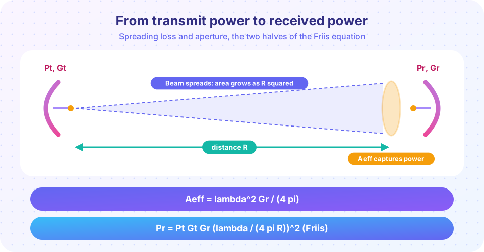
A transmitter of power Pt feeding an antenna of gain Gt creates, at distance R in the beam direction, a power density
S = Pt Gt / (4π R²)
The product Pt Gt is the EIRP. A 1 W transmitter with a 10 dBi antenna has an EIRP of 10 W; regulators limit EIRP, not just conducted power. The 4π R² is the area of a sphere: the same power is spread over a surface that grows as R². Doubling the distance quarters the density (6 dB less).
Effective aperture
A receiving antenna absorbs Pr = S · Aeff. Reciprocity ties Aeff to the gain:
Aeff = λ² Gr / (4π)
Two consequences are worth remembering.
- At a given frequency, higher gain means larger effective aperture. For a dish,
Aeff = η A, with η typically 0.5 to 0.7, givingG = η (π D / λ)². - At a given gain, the aperture shrinks with frequency squared. An isotropic antenna (G = 1) at 2.4 GHz has
Aeff = λ²/(4π) = 0.1249² / 12.566 ≈ 12.4 cm²; at 24 GHz it is 100 times smaller. This is the physical reason higher frequencies lose more in free space even though nothing is absorbed: for fixed-gain antennas, they simply collect less.
The Friis transmission equation
Combine the two:
Pr = S · Aeff = Pt Gt Gr (λ / (4π R))²
The bracket is 1/FSPL per isotropic antenna. In decibels, using the free-space path loss L_fs = 20 log10(4π R / λ):
Pr (dBm) = Pt (dBm) + Gt (dBi) + Gr (dBi) - L_fs (dB)
Practical form for frequency in MHz and distance in km: L_fs = 32.44 + 20 log10(f_MHz) + 20 log10(d_km). Every doubling of distance or of frequency adds 6.02 dB.
Worked example. A 2.4 GHz access point (Pt = 20 dBm, Gt = 3 dBi) serves a laptop (Gr = 0 dBi) 50 m away.
λ = 0.1249 m.L_fs = 20 log10(4π · 50 / 0.1249) = 20 log10(5030) = 74.0 dB.Pr = 20 + 3 + 0 - 74.0 = -51.0 dBm.
Check with the other form: 32.44 + 20 log10(2400) + 20 log10(0.05) = 32.44 + 67.60 - 26.02 = 74.0 dB ✓.
When the equation applies
Friis assumes free space, polarization match, impedance match, and far-field separation: R > 2 D²/λ for antennas of largest dimension D. For a 1 m dish at 10 GHz that is 66.7 m; closer than that, the field is in the near zone and the formula overestimates gain. In real links add terms for mismatch, polarization loss, atmospheric absorption (rain, oxygen, water vapor) and obstacles; the next chapter develops them.
Common misconceptions
"Higher frequency means the wave loses more energy in free space." Free space is lossless. The extra "loss" at higher frequency is the smaller aperture of a fixed-gain antenna. If you keep antenna sizes fixed instead, the gains rise and the link gets better.
"Pr falls as 1/R." Power falls as 1/R²; field strength falls as 1/R.
"I can apply Friis at 10 cm." Not for large antennas: near-field effects dominate.
Try it
Press Run (or Ctrl + Enter) to see the result here.
Program input · what you'd type while the program runs
Type the answers before you press Run, one per line. Each time the program reads a line (with input()), it gets the next line from this box.
Press Run (or Ctrl + Enter) to see the result here.
Program input · what you'd type while the program runs
Type the answers before you press Run, one per line. Each time the program reads a line (with input()), it gets the next line from this box.
Press Run (or Ctrl + Enter) to see the result here.
Program input · what you'd type while the program runs
Type the answers before you press Run, one per line. Each time the program reads a line (with input()), it gets the next line from this box.
Check your understanding
Quick check · 5 questions
of 5 answered You scored / 5 · perfect!
-
1. The distance between two antennas is doubled. Received power (free space) changes by
Pr is proportional to 1/R^2, so doubling R costs 6 dB. -
2. A transmitter delivers 5 W (37 dBm) to an antenna of gain 12 dBi. The EIRP is
EIRP = 37 + 12 = 49 dBm, about 79 W. -
3. What does the effective aperture of an isotropic antenna depend on?
With G = 1, Aeff = lambda^2/(4 pi). -
4. Path loss between isotropic antennas at 2.4 GHz and 10 m is about
32.44 + 67.6 + 20 log10(0.01) = 32.44 + 67.6 - 40 = 60.0 dB. -
5. Why is Friis not valid at very short distances?
Friis assumes far-field conditions, R > 2D^2/lambda.
Summary
S = EIRP/(4πR²)andPr = S AeffwithAeff = λ²G/(4π).- Friis:
Pr = Pt Gt Gr (λ/(4πR))², or in dBPt + Gt + Gr - L_fs. L_fs = 32.44 + 20 log10(f_MHz) + 20 log10(d_km); +6 dB per doubling of distance or frequency.- Check the far-field condition
R > 2D²/λ.
Next: Chapter review
Track your progress
Create a free account to tick off lessons and pick up where you left off on any device.
of RF Engineering and Antennas lessons completed