


















Lesson 11 of 46 · Smith Chart and Matching
Chapter 3 Overview: The Smith Chart and Impedance Matching
A map of chapter 3: what the Smith chart shows, why RF engineers still use it, and how you will use it to read impedances, move along lines and design matching networks.
In 1939 Phillip H. Smith, an engineer at RCA, was tired of grinding through complex-number formulas to design antenna matching sections. He drew a chart that turned the whole calculation into geometry, and the Smith chart has been in use ever since. Today software does the arithmetic, yet engineers still reach for the chart because it shows at a glance what a network is doing, where a trace is heading and how much room there is to match it.
This chapter teaches you to read the chart as a picture of reflection coefficients and then to use it to design matching networks. The earlier chapter gave you the formulas; here they become shapes.
What you will learn
- What the Smith chart represents and how it relates to the reflection coefficient.
- What the chart will let you do: read VSWR, rotate along a line, convert between impedance and admittance.
- The matching methods that follow: lumped L-networks, quarter-wave sections and stubs.
- How this chapter prepares you for the S-parameter plots of chapter 4.
One chart, two views
Same point, two readings.
Moving on the chart
Each step is one picture.
Matching tools
All three end at the center.
The big picture
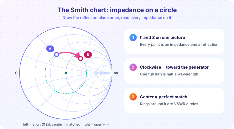
Every passive impedance has a reflection coefficient with magnitude at most 1. Plot the real and imaginary parts of Γ and every passive load falls inside a circle of radius 1: the Γ-plane. The Smith chart is that plane with a grid of impedance circles drawn on top. Instead of coordinates for Γ, you read off r and x, the resistance and reactance divided by Z0.
Three facts make the chart powerful:
- The center is a perfect match (
Γ = 0,z = 1). The left edge of the real axis is a short circuit, the right edge an open circuit. - The upper half of the chart is inductive (
+jx) and the lower half capacitive (−jx). - On a lossless line a mismatch keeps its
|Γ|and only rotates, so a transmission line is a circular arc on the chart.
Matching then becomes a path-finding problem: start at the load, take steps (add a series part, a shunt part, a length of line) until you reach the center.
What each lesson covers
- Smith chart basics: normalization, where the circles come from, reading a point, VSWR circles and the admittance chart.
- Lumped-element matching: the L-network, its Q, low-pass and high-pass versions, and bandwidth.
- Stub and quarter-wave matching: single-stub design with numbers and the λ/4 transformer.
- Chapter 3 review: one-page summary and quiz.
Try it
The Smith chart is more than a classroom drawing. Engineers see the impedance of an antenna or a circuit across frequency as a trace on it. Here is a series resonant circuit (50 Ω, 10 nH and 2.533 pF) swept from 700 MHz to 1.3 GHz. Its resistance stays at 50 Ω, which is the r = 1 circle, while the reactance sweeps from capacitive through zero (at 1 GHz) to inductive. Watch the trace follow the circle.
Press Run (or Ctrl + Enter) to see the result here.
Program input · what you'd type while the program runs
Type the answers before you press Run, one per line. Each time the program reads a line (with input()), it gets the next line from this box.
The second tool shows the map from impedance to reflection coefficient. A grid of impedances (constant r lines and constant x lines in the impedance plane) is drawn as circles after the transformation Γ = (z − 1)/(z + 1). That is the entire secret of the Smith chart.
Press Run (or Ctrl + Enter) to see the result here.
Program input · what you'd type while the program runs
Type the answers before you press Run, one per line. Each time the program reads a line (with input()), it gets the next line from this box.
Check your understanding
Quick check · 4 questions
of 4 answered You scored / 4 · perfect!
-
1. Where is a perfectly matched load on the Smith chart?
Γ = 0 and z = 1 plot at the center. -
2. Which half of the chart shows inductive impedances?
Positive reactance (+jx) is in the upper half. -
3. What does moving toward the generator along a lossless line do to a point?
|Γ| is constant on a lossless line; only the phase changes, clockwise toward the generator. -
4. Who introduced the chart and when?
Phillip H. Smith of RCA published the chart in 1939.
Summary
- The Smith chart is the reflection-coefficient plane with impedance circles drawn on it.
- Center = matched, left = short, right = open, upper = inductive, lower = capacitive.
- A lossless line is a clockwise arc; a mismatch keeps its
|Γ|. - The chapter covers reading the chart, L-networks, stubs and quarter-wave sections.
Next: Smith Chart Basics
Track your progress
Create a free account to tick off lessons and pick up where you left off on any device.
of RF Engineering and Antennas lessons completed