


















Lesson 37 of 49 · Spectroscopy
UV-Visible Spectroscopy and the Beer-Lambert Law
Understand electronic transitions, color and fluorescence, derive the Beer-Lambert law, and use calibration curves to find concentrations from absorbance.
Why is a copper sulfate solution blue and chlorophyll green? Why does a quinine solution glow under ultraviolet light? Why can a hospital lab measure a drug concentration in blood in seconds? All of these rest on electronic spectroscopy: absorption of ultraviolet or visible light promotes an electron from one orbital to another. The energies, 1.5 to 6 eV, are far larger than vibrational or rotational ones, and the technique is the workhorse of quantitative analysis because the absorbance is directly proportional to concentration.
What you will learn
- Name the common electronic transitions and relate color to absorbed wavelength
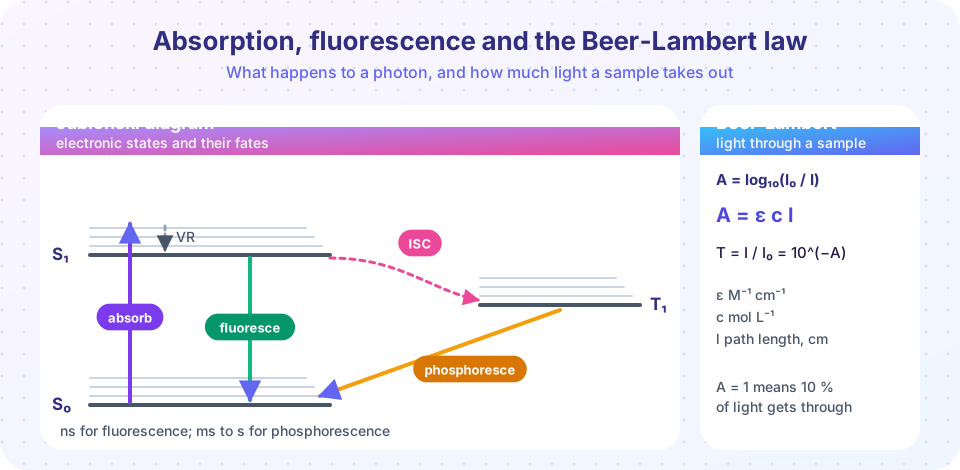
- Explain absorption, fluorescence and phosphorescence with a Jablonski diagram
- Use
A = εcland the relation between A and transmittance - Build and use a calibration curve
Key terms
Chromophore: the part of a molecule that absorbs UV or visible light, typically a conjugated π system.
Absorbance (A): A = log₁₀(I₀/I), the logarithm of the ratio of incident to transmitted intensity.
Molar absorption coefficient (ε): a property of a substance at a given wavelength, in M⁻¹ cm⁻¹.
Franck–Condon principle: electronic transitions happen so fast that nuclei do not move during them ("vertical" transitions).
Electronic transitions
An electron is promoted from an occupied orbital to an empty one. Common types, in order of increasing energy:
| Transition | Typical wavelength | Example |
|---|---|---|
| n → π* | 270–350 nm | the C=O of acetone (weak, ε about 10–100) |
| π → π* | 160–250 nm for isolated bonds, longer with conjugation | ethene, benzene, dyes (strong, ε of 10³ to 10⁵) |
| n → σ* | 170–260 nm | alcohols, amines |
| σ → σ* | below 150 nm | alkanes |
As the box model suggested, longer conjugation lowers the gap, moving absorption to longer wavelength. β-carotene absorbs blue light near 450 nm and so looks orange. Transition-metal complexes are colored by d–d transitions, where an electron moves between d orbitals split by the ligands: hydrated copper(II) absorbs red-orange light and looks blue.
Color rule: the color you see is roughly the complement of what is absorbed. Absorb violet and the solution looks yellow-green; absorb red and it looks blue-green.
The Franck–Condon principle and band shape
Electrons move far faster than nuclei, so absorption occurs at the ground-state geometry and leaves the molecule in an excited electronic state with a bond length that is wrong for it. The molecule usually lands on an excited vibrational level, and the result is a broad band with a vibrational fine structure in gases or rigid solvents, merged into a smooth hump in solution.
What happens next: the Jablonski diagram
After absorption, in the S₀ → S₁ transition, the molecule can
- relax vibrationally to the bottom of S₁ within picoseconds, giving heat to the solvent;
- emit light and return to S₀: fluorescence, in nanoseconds, at a longer wavelength than the absorbed light (the Stokes shift);
- cross to a triplet state T₁ by intersystem crossing, and from there emit slowly: phosphorescence, in milliseconds to seconds, because the T₁ → S₀ transition is spin-forbidden (glow-in-the-dark materials);
- return to S₀ without emitting light (internal conversion), or take part in a photochemical reaction.
The fluorescence quantum yield Φ_F is the fraction of absorbed photons that are re-emitted as fluorescence. Fluorescent dyes and probes used in microscopy have yields approaching one.
The Beer–Lambert law
Slice the sample into thin layers of thickness dl. Each layer absorbs a fraction of the light proportional to its concentration c, so dI = −κ c I dl. Integrating gives an exponential decay, conventionally written in base 10:
A = log₁₀(I₀ / I) = ε c l
with ε in M⁻¹ cm⁻¹, c in mol L⁻¹ and path length l in cm. The transmittance is T = I/I₀ = 10^(−A). Useful anchor points: A = 0 means no absorption, A = 1 means 10 % transmitted, A = 2 means 1 %.
Worked examples
- A solution with
A = 0.435transmitsT = 10^(−0.435) = 0.367, or 36.7 %. - A dye has
ε = 1.2 × 10⁴ M⁻¹ cm⁻¹. A 1.00 cm cuvette readsA = 0.60. Thenc = A/(εl) = 0.60 / (1.2×10⁴ × 1.00) = 5.0 × 10⁻⁵ M. - If you dilute that solution by a factor of 4, A falls to 0.15 (because c is divided by 4); if you use a 0.25 cm cuvette instead, the same.
Calibration curves and practical limits
Real analysis does not rely on a literature ε. Instead, measure the absorbance of standards of known concentration, plot A against c, and fit a straight line (the slope is εl). Then read the unknown's concentration from the line.
Practical rules:
- Work with absorbances between about 0.1 and 1: very low values are noisy, very high values let stray light dominate.
- Use a blank (solvent only) to set A = 0.
- The law fails at high concentration (molecules interact, refractive index changes), with scattering samples (turbid solutions) and when the absorber takes part in an equilibrium such as an acid–base indicator, whose form changes with dilution.
- With several absorbers, absorbances add:
A = (ε₁c₁ + ε₂c₂) l, so measuring at two wavelengths solves for two concentrations.
Common misconceptions
"Absorbance is the fraction of light absorbed." That would be 1 − T. Absorbance is the base-10 logarithm of 1/T, and it is the quantity that is proportional to concentration.
"A doubled concentration halves the transmittance." It squares it: T = 10^(−A) and doubling A squares T.
"Fluorescence has the same wavelength as the absorbed light." It is shifted to longer wavelengths because energy is lost in relaxation first.
Try it
First, a virtual cuvette. Move the sliders and watch the light intensity transmitted and the absorbance. It is a calculator with a graphic, using ε = 1.2 × 10⁴ M⁻¹ cm⁻¹.
Second, a complete calibration. The standards are invented for the exercise (true ε = 15 000 M⁻¹ cm⁻¹, 1.00 cm cuvette, instrument noise 0.005 in A); the unknown reads A = 0.320.
Press Run (or Ctrl + Enter) to see the result here.
Program input · what you'd type while the program runs
Type the answers before you press Run, one per line. Each time the program reads a line (with input()), it gets the next line from this box.
Check your understanding
Quick check · 5 questions
of 5 answered You scored / 5 · perfect!
-
1. A solution has absorbance 2.0. What fraction of the light is transmitted?
T = 10⁻² = 0.01. -
2. ε = 8000 M⁻¹ cm⁻¹, l = 1 cm and A = 0.40. What is c?
c = A/(εl) = 0.40/8000 = 5.0 × 10⁻⁵ M. -
3. Why is fluorescence emitted at longer wavelength than absorption?
That is the Stokes shift. -
4. Which transition is typically the weakest (smallest ε)?
n → π* transitions are symmetry-forbidden to a large extent and have ε around 10–100. -
5. Phosphorescence lasts much longer than fluorescence because
Triplet-to-singlet transitions require a spin flip, which is slow.
Summary
- Electronic transitions (n → π*, π → π*, d–d) give color; longer conjugation means longer wavelength.
- Jablonski diagram: absorption, vibrational relaxation, fluorescence (ns), intersystem crossing and phosphorescence (ms–s).
A = log₁₀(I₀/I) = εclandT = 10^(−A); absorbances add for mixtures.- Calibration curves convert measured absorbance into concentration; stay between A ≈ 0.1 and 1.
Next: NMR spectroscopy
Track your progress
Create a free account to tick off lessons and pick up where you left off on any device.
of Physical Chemistry lessons completed