


















Lesson 44 of 49 · Projects and Practice
Project: Predict a Shelf Life from Hot-Storage Data
A hands-on kinetics project: fit decay curves at four temperatures, build an Arrhenius plot, extrapolate to room temperature and predict a shelf life with an uncertainty range.
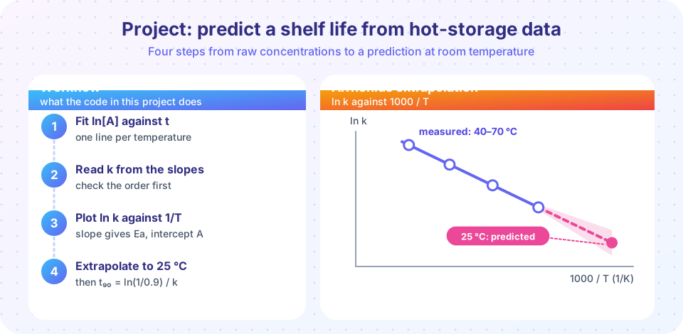
Companies cannot wait two years to learn how long a medicine will last, so they store samples at raised temperatures and extrapolate. The method is applied kinetics: measure how fast the active ingredient decays at 40, 50, 60 and 70 °C, find the activation energy, and use the Arrhenius equation to predict the rate at room temperature. In this project you will do exactly that with data that we generate, so that you know the true answer and can judge how well the analysis performs.
What you will learn
- Test the order of a decay and fit a rate constant at each temperature
- Build an Arrhenius plot and extract Ea and A with uncertainties
- Extrapolate to a storage temperature and compute
t₉₀ - Recognize the limits of extrapolation
Key terms
Shelf life (t₉₀): the time for the active ingredient to fall to 90 % of its labeled amount; for a first-order decay, t₉₀ = ln(1/0.9)/k = 0.1054/k.
Accelerated testing: measuring at elevated temperature to learn about slow changes at normal temperature.
Extrapolation: predicting outside the measured range; its uncertainty grows with distance from the data.
Confidence band: the range of lines consistent with the data at a stated confidence. With only four points the multiplier is the Student t value (about 4.3), not 2.
The scenario
A tablet's active ingredient breaks down by a first-order process. All the data below are simulated: we choose a true activation energy of 85 kJ mol⁻¹ and a true rate constant of 3.0 × 10⁻⁴ day⁻¹ at 25 °C, add 1 % random scatter to each measurement, and pretend not to know the answers. Concentration is expressed as a percentage of the labeled amount at times 0, 7, 14, 28, 56, 90, 120 and 180 days.
Step 1: what order is it?
Before fitting anything, check the order at one temperature (60 °C) using the three linear plots from Chapter 5.
Press Run (or Ctrl + Enter) to see the result here.
Program input · what you'd type while the program runs
Type the answers before you press Run, one per line. Each time the program reads a line (with input()), it gets the next line from this box.
The first-order plot should give the straightest line. If more than one order looks acceptable, collect data further into the reaction or use half-life tests, as in Chapter 5.
Step 2: rate constants, Arrhenius plot and prediction
Now simulate all four temperatures, fit ln C against t to get each k, then fit ln k against 1/T. The fit returns the covariance of its coefficients, which lets us put an uncertainty on the extrapolated k at 25 °C.
Press Run (or Ctrl + Enter) to see the result here.
Program input · what you'd type while the program runs
Type the answers before you press Run, one per line. Each time the program reads a line (with input()), it gets the next line from this box.
Step 3: critical reading
Look at what the analysis gave and ask the questions an experienced chemist would ask.
- How close is the Ea estimate to the truth, and how large is its uncertainty? Read the printed standard error: with only four temperatures spanning 30 K it is not negligible, and an error in Ea is multiplied by the distance of the extrapolation.
- How far did we extrapolate? From 40 °C down to 25 °C is 15 K outside the lowest measured point. The band widens rapidly outside the data.
- Is the Arrhenius model valid? In real formulations, melting, glass transitions, humidity or a change of mechanism between 40 and 70 °C can make the plot curve. If it does, the prediction is not trustworthy.
- Are all the points equally reliable? The 40 °C data lose only a small fraction of the drug within 180 days, so their k values are the hardest to pin down, yet they sit closest to the target. Proper stability studies treat this carefully and confirm predictions with real-time data.
Never use a model like this to decide the safety of a real product. The project is an exercise in method; regulators require validated procedures and real-time data.
Extensions to try
- Change the noise from 1 % to 3 % and see how the uncertainty of the shelf life grows.
- Use only three temperatures (50, 60, 70 °C) and compare the prediction with the four-point analysis.
- Replace the first-order decay with a second-order one and repeat the analysis of the order at each temperature.
- Switch to an Eyring analysis by plotting
ln(k/T)against1/Tand extract ΔH‡ and ΔS‡.
Check your understanding
Quick check · 4 questions
of 4 answered You scored / 4 · perfect!
-
1. For a first-order decay, t₉₀ is
t₉₀ = ln(1/0.9)/k = 0.1054/k. -
2. Why is extrapolating an Arrhenius plot to a temperature far below the data risky?
Both statistical and systematic errors increase with distance from the measured range. -
3. The slope of the Arrhenius plot ln k against 1000/T is −10.2. What is Ea?
Ea = 10.2 × 1000 × 8.314 = 85 kJ/mol. -
4. If the true half-life at 70 °C is 26 days, which fraction remains after 52 days?
Two half-lives: (1/2)² = 25 %.
Summary
- Fit the right order first, then extract k at each temperature.
ln kagainst1/Tgives Ea; extrapolation gives k at the storage temperature andt₉₀ = 0.1054/k.- Report an uncertainty range, check the Arrhenius assumption and never extrapolate blindly.
Track your progress
Create a free account to tick off lessons and pick up where you left off on any device.
of Physical Chemistry lessons completed