


















Lesson 4 of 49 · Getting Started
The mathematics toolkit: logs, slopes, areas and straight lines
Refresh the mathematics used in physical chemistry: exponentials and logarithms, derivatives, partial derivatives, integrals and straight-line fits, with Python examples.
Physical chemistry uses surprisingly little mathematics, but it uses the same few ideas again and again. Exponentials and logarithms describe rates and equilibria. Derivatives describe how one quantity changes with another. Integrals add up small contributions. And straight-line graphs turn messy data into constants such as activation energies.
This lesson refreshes exactly those tools, with chemistry examples, so later chapters can move quickly.
What you will learn
- The properties of exponentials and natural logarithms.
- What a derivative and a partial derivative measure.
- How an integral gives work and heat from a curve.
- How to linearize an equation and fit a straight line.
Key terms
Natural logarithm (ln): the inverse of the exponential, ln(e^x) = x.
Derivative: the slope of a curve at a point, dy/dx.
Partial derivative: the slope with respect to one variable while the others are held constant, written (∂y/∂x) with the fixed variables as subscripts.
Integral: the area under a curve, the sum of many small pieces.
Linearization: rewriting an equation as y = mx + c so data fall on a straight line.
Exponentials and logarithms
The number e = 2.71828... is the base for which the slope of e^x equals e^x. This is why it describes processes whose rate is proportional to the amount present: radioactive decay, first-order reactions, Boltzmann populations.
Rules you will use constantly:
| Rule | Example |
|---|---|
ln(ab) = ln a + ln b |
ln(6) = ln 2 + ln 3 |
ln(a/b) = ln a - ln b |
ln(K2/K1) |
ln(a^n) = n ln a |
ln(P^2) = 2 ln P |
e^(a+b) = e^a e^b |
|
ln(e^x) = x |
Two practical points. First, you can only take the logarithm of a dimensionless number. When you see ln P in a textbook it really means ln(P/P°), with a standard pressure P° dividing out the unit. Second, converting between ln and log₁₀ uses ln x = 2.303 log₁₀ x.
Worked example. A first-order reaction has c = c₀ e^(-kt) with k = 0.0231 min⁻¹. When has half the reactant gone? Set c/c₀ = 1/2: ln(1/2) = -kt, so t = ln 2 / k = 0.693 / 0.0231 = 30.0 min.
Derivatives
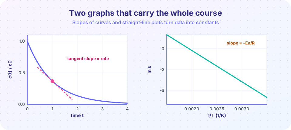
If y depends on x, then dy/dx is the slope of the graph. Chemistry examples are everywhere: the rate of reaction is the slope of a concentration-time curve, the heat capacity is the slope of energy against temperature.
The rules you need:
d(x^n)/dx = n x^(n-1)d(e^(ax))/dx = a e^(ax)d(ln x)/dx = 1/x- sum, product and chain rules as usual.
Example. Pressure of an ideal gas as a function of volume at fixed T: P = nRT/V. Then dP/dV = -nRT/V²: pressure drops more steeply at small volume.
Partial derivatives
Most thermodynamic quantities depend on several variables. The ideal gas pressure is a function of n, T and V: P(n, T, V) = nRT/V. A partial derivative asks how P changes with one variable while holding the others fixed:
(∂P/∂T) at constant V and n = nR/V
(∂P/∂V) at constant T and n = -nRT/V²
The total change when several variables change a little is the sum of the contributions:
dP = (∂P/∂T) dT + (∂P/∂V) dV
This "total differential" is the model for every thermodynamic relation in the course, for example dU = (∂U/∂T)_V dT + (∂U/∂V)_T dV. A quantity that has such a differential, depending only on the state, is a state function (chapter 2). The order of differentiation does not matter for state functions: ∂²f/∂x∂y = ∂²f/∂y∂x. This simple fact gives the Maxwell relations that you will meet later.
Integrals
An integral is a sum of many small slices. Work done by a gas expanding against pressure P is w = -∫ P dV. For an ideal gas at constant temperature P = nRT/V, so
w = -nRT ∫ dV/V from V1 to V2 = -nRT ln(V2/V1)
The only integrals needed in this course are of the forms ∫ x^n dx, ∫ dx/x = ln x, and ∫ e^(ax) dx = e^(ax)/a. When an integral gets harder, we let NumPy do it numerically.
Linearizing: the secret of reading constants
Many laws are not straight lines, but a clever choice of axes makes them straight. If y = mx + c, then the slope gives m and the intercept gives c directly.
| Equation | Plot | Slope | Intercept |
|---|---|---|---|
k = A e^(-Ea/RT) |
ln k against 1/T |
-Ea/R |
ln A |
ln[A] = ln[A]₀ - kt |
ln[A] against t |
-k |
ln[A]₀ |
1/[A] = 1/[A]₀ + kt |
1/[A] against t |
k |
1/[A]₀ |
ln K = -ΔH°/RT + ΔS°/R |
ln K against 1/T |
-ΔH°/R |
ΔS°/R |
PV = nRT |
V against T at fixed P |
nR/P |
0 |
We will meet every one of these. The method is always the same: take the equation, take logs if needed, identify y, x, m, c.
Fitting a line
Real data scatter, so we fit a line by least squares, choosing the slope and intercept that minimize the sum of squared vertical distances. NumPy does it with np.polyfit(x, y, 1). Always plot the data with the fit: a good R² hides curvature if you never look.
Worked example: activation energy from data
At 300 K a rate constant is 0.0020 s⁻¹ and at 320 K it is 0.0155 s⁻¹. Find Ea.
ln(k2/k1) = (Ea/R)(1/T1 - 1/T2), so Ea = R ln(k2/k1) / (1/T1 - 1/T2).
ln(0.0155/0.0020) = ln 7.75 = 2.0481/300 - 1/320 = 0.0033333 - 0.003125 = 2.0833 x 10⁻⁴ K⁻¹Ea = 8.3145 x 2.048 / 2.0833e-4 = 8.17 x 10⁴ J/mol = 81.7 kJ/mol
Common misconceptions
"The log of a quantity with units is fine." Only dimensionless arguments belong in ln; divide by a reference value first.
"The slope of a plot is the same as the ratio of two points." Only for a straight line through the origin. Use a fit or two well-separated points.
"ln means log base 10." In science ln is base e and log is usually base 10; check which.
"A partial derivative holds nothing constant." The variables you hold fixed are part of its meaning and are always written as subscripts.
Try it
First, differentiate and integrate symbolically with SymPy. Here we recover the isothermal work formula.
Press Run (or Ctrl + Enter) to see the result here.
Program input · what you'd type while the program runs
Type the answers before you press Run, one per line. Each time the program reads a line (with input()), it gets the next line from this box.
Next, a linear fit. The program generates noisy Arrhenius data (a labelled simulation with a made-up Ea of 80 kJ/mol), fits ln k against 1/T and recovers the activation energy.
Press Run (or Ctrl + Enter) to see the result here.
Program input · what you'd type while the program runs
Type the answers before you press Run, one per line. Each time the program reads a line (with input()), it gets the next line from this box.
Check your understanding
Quick check · 5 questions
of 5 answered You scored / 5 · perfect!
-
1. A first-order reaction has k = 0.0231 min^-1. What is its half-life?
t1/2 = ln 2 / k = 0.693 / 0.0231 = 30.0 min. -
2. What is (dP/dV) at constant T for P = nRT/V?
Differentiate nRT V^-1 to get -nRT V^-2. -
3. Plotting ln k against 1/T gives a straight line. What does the slope equal?
ln k = ln A - (Ea/R)(1/T), so the slope is -Ea/R. -
4. Which statement about the argument of a logarithm is correct?
Logarithms and exponentials need dimensionless arguments, so divide by a reference value. -
5. The work of isothermal reversible expansion of an ideal gas from V1 to V2 is
w = -integral of nRT/V dV = -nRT ln(V2/V1).
Summary
lnandexpare inverses; useln(ab) = ln a + ln bandln(a^n) = n ln a; arguments must be dimensionless.- A derivative is a slope; a partial derivative holds the other variables fixed.
- A total differential adds the partial contributions:
dP = (∂P/∂T)dT + (∂P/∂V)dV. - Integrals add small pieces: isothermal ideal-gas work is
-nRT ln(V2/V1). - Linearize equations so slopes and intercepts are the constants you want, then fit and plot.
Next: Chapter 1 review
Track your progress
Create a free account to tick off lessons and pick up where you left off on any device.
of Physical Chemistry lessons completed