


















Lesson 43 of 46 · Projects and Practice
Project: estimate how long antibody protection lasts
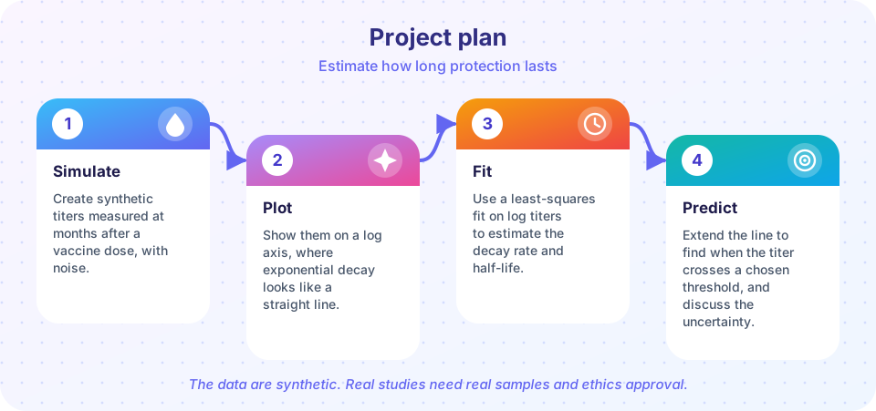
Simulate noisy antibody titers after vaccination, fit an exponential decay on a log scale, estimate the half-life, and predict when the level crosses a threshold.
Serologists measure antibody levels in blood samples taken at different times after a vaccine dose. When the points are plotted on a log scale, they often fall roughly along a straight line, because antibody levels decline by a constant fraction in each period, which is exponential decay. The slope of the line gives the half-life, the time over which the level halves.
In this project you will go through the whole workflow in Python: make synthetic data, plot it, fit a model, and use it to predict when the level will cross a chosen threshold. You will also see how uncertain such a prediction is. The data here are synthetic, generated by a program, and the numbers do not describe any real vaccine. Real studies require real samples, consent and ethical review.
What you will learn
- Why antibody decay is straight on a log plot.
- How to fit a line to log-transformed data and convert the slope to a half-life.
- How to predict the time to reach a threshold.
- How to use resampling to show uncertainty.
Key terms
Titer: a measure of antibody concentration. Here, arbitrary units.
Half-life: the time for a quantity to fall to half its value.
Exponential decay: decline by the same fraction in each equal time interval.
Least squares: a method that chooses the line minimizing the squared differences from the data.
Bootstrap: resampling the data with replacement to see how much an estimate varies.
Step 1: simulate the data
Suppose the true half-life is 180 days and the level one month after the dose is 1,200 arbitrary units. Real measurements are noisy, and the noise from assays is often proportional, so the logarithm of the level has roughly constant scatter. We simulate this by adding normal noise to the log level.
The model is level(t) = L0 × 2^(−t / h), so log2(level) = log2(L0) − t / h. A straight-line fit of log2(level) against time has slope −1/h.
Press Run (or Ctrl + Enter) to see the result here.
Program input · what you'd type while the program runs
Type the answers before you press Run, one per line. Each time the program reads a line (with input()), it gets the next line from this box.
Step 2: fit the decay
Taking the base-2 logarithm turns the model into a straight line. NumPy's polyfit finds the least-squares line, and the half-life is the negative inverse of the slope.
Press Run (or Ctrl + Enter) to see the result here.
Program input · what you'd type while the program runs
Type the answers before you press Run, one per line. Each time the program reads a line (with input()), it gets the next line from this box.
Step 3: predict the time to a threshold
Suppose a certain level, say 100 units, is taken as a protective threshold. This is an assumption made for the exercise. For real pathogens, protective levels depend on the antibody test and the infection, and some have no agreed threshold. With the fitted line, the time when the level reaches the threshold satisfies log2(threshold) = slope × t + intercept.
Because we have only ten noisy points, the estimate carries uncertainty. A bootstrap resamples the measurements with replacement many times, refits each time, and reports the spread of predictions.
Press Run (or Ctrl + Enter) to see the result here.
Program input · what you'd type while the program runs
Type the answers before you press Run, one per line. Each time the program reads a line (with input()), it gets the next line from this box.
Choosing the threshold and reading the answer
The threshold in step 3 is the most arbitrary number in the project. For some infections there is a measured level of antibody that predicts protection in studies, called a correlate of protection. For others there is none, or the level depends on the laboratory method. When you read a statement such as "protection lasts X years", ask which threshold was used and where it came from. Try changing the threshold from 100 to 200 and to 50 in the code and watch how the predicted time moves: halving the threshold adds exactly one half-life, which is a useful rule of thumb because each halving of the level takes one half-life.
Notice too how the width of the bootstrap interval depends on the noise. In real studies, a wide interval is a sign that more samples, more time points or more people are needed before drawing conclusions.
Discussion: what this project does and does not show
What it shows. Log plots turn exponential decay into lines, a fitted slope gives a half-life, and a threshold turns the half-life into a time. A resampling method puts error bars on the answer and reminds you that precise-looking numbers can be fragile.
What it ignores. Real antibody decay is often not a single exponential. Many studies find a fast fall in the first months, as short-lived plasma cells die, followed by a slow decline governed by long-lived plasma cells. Fitting one straight line through early data can overestimate how quickly protection is lost. Real antibody levels also vary between people, so a population average hides a wide spread. Antibody levels are only one part of protection, because memory B and T cells can respond to exposure even when antibodies are low.
Extension ideas. Fit two exponentials and compare. Change the noise and the number of sample times and see how wide the interval becomes. Add several simulated people with different half-lives and plot the distribution of times to the threshold. Try different thresholds.
Check your understanding
Quick check · 4 questions
of 4 answered You scored / 4 · perfect!
-
1. Why do exponential decay data appear as a straight line on a log plot?
A constant fractional decline means the log of the level falls by a constant amount. -
2. A fitted line of log2(level) against days has slope -0.004 per day. What is the half-life?
Half-life = -1/slope = 1/0.004 = 250 days. -
3. What does a bootstrap show?
Resampling and refitting give a distribution of estimates, from which an interval can be taken. -
4. Why might a single exponential fit overestimate how quickly protection is lost?
Decay is often biphasic: a fast early phase followed by a slower phase.
Summary
- On a log scale, exponential decay of antibody is a straight line whose slope gives the half-life.
- A fitted line and a threshold give a predicted time to cross, and a bootstrap shows its uncertainty.
- Real decay is often biphasic, and antibody level is only one part of protection.
- The data in this project are synthetic and for learning only.
Track your progress
Create a free account to tick off lessons and pick up where you left off on any device.
of Immunology lessons completed